R
Getting started
Examples using the 84.51 data set.
Please see https://piazza.com/class/kdrxb6dxa8c6by?cid=110 for example code, to go along with this video.
Please see https://piazza.com/class/kdrxb6dxa8c6by?cid=110 for example code, to go along with this video.
We read in the data from the 8451 data set (This is not the same data set from Project 2! It is only intended to give you an idea about how to use basic functions in R!) The read.csv function is used to read in a data frame. The variable myDF will be a data frame that stores the data.
myDF <- read.csv("/class/datamine/data/8451/The_Complete_Journey_2_Master/5000_transactions.csv")Please give the data frame a minute or two, to load. It is big!
The data frame has 10625553 rows and 9 columns:
dim(myDF)## [1] 1000000 9This is the data that describes the first 6 purchases:
head(myDF)## BASKET_NUM HSHD_NUM PURCHASE_ PRODUCT_NUM SPEND UNITS STORE_R WEEK_NUM YEAR
## 1 24 1809 03-JAN-16 5817389 -1.50 -1 SOUTH 1 2016
## 2 24 1809 03-JAN-16 5829886 -1.50 -1 SOUTH 1 2016
## 3 34 1253 03-JAN-16 539501 2.19 1 EAST 1 2016
## 4 60 1595 03-JAN-16 5260099 0.99 1 WEST 1 2016
## 5 60 1595 03-JAN-16 4535660 2.50 2 WEST 1 2016
## 6 168 3393 03-JAN-16 5602916 4.50 1 SOUTH 1 2016Similarly, these are the amounts spent on the first 6 purchases. We use the dollar sign to pull out a specific column of the data and focus (only) on that column.
head(myDF$SPEND)## [1] -1.50 -1.50 2.19 0.99 2.50 4.50These first 6 values in the SPEND column add up to a total sum of 7.18 (you can check by hand if you like!)
sum(head(myDF$SPEND))## [1] 7.18The average of the first 6 values in the SPEND column is 1.196667
mean(head(myDF$SPEND))## [1] 1.196667The first 100 values in the SPEND column are:
head(myDF$SPEND, n=100)## [1] -1.50 -1.50 2.19 0.99 2.50 4.50 3.49 2.79 1.00 9.98 1.29 1.79
## [13] 3.99 1.00 2.00 10.80 3.49 1.00 3.99 1.88 0.49 2.49 1.99 2.50
## [25] 1.67 1.99 5.50 7.89 6.49 1.00 2.78 3.69 1.19 0.69 3.00 5.99
## [37] 8.19 3.49 4.29 5.66 0.99 5.99 0.99 8.11 12.82 7.99 4.19 1.49
## [49] 4.96 3.49 4.49 2.79 2.99 5.49 3.99 12.00 3.79 0.89 4.99 2.29
## [61] 1.69 5.78 6.99 2.00 3.89 6.77 2.69 4.99 3.20 14.40 6.93 2.50
## [73] 1.00 5.98 1.75 1.19 4.25 3.00 1.11 0.98 8.17 13.10 17.98 4.38
## [85] 5.79 3.59 4.99 11.56 3.42 2.99 17.99 1.50 -0.38 3.14 2.49 3.99
## [97] 3.39 1.49 0.53 1.25Note that, in the line above, we have an "index" at the far left-hand side of the Console. It shows the position of the first value on each line. The values will change, depending on how wide your screen is.
Here is the 1st value in the SPEND column:
myDF$SPEND[1]## [1] -1.5Here is the 22nd value in the SPEND column:
myDF$SPEND[22]## [1] 2.49Here is the 25th value in the SPEND column:
myDF$SPEND[25]## [1] 1.67Here are the last 20 values in the SPEND column. (Notice that we changed head to tail, since tail refers to the end rather than the start.)
tail(myDF$SPEND, n=20)## [1] 1.00 1.39 19.98 2.97 0.89 2.89 5.99 1.79 1.99 1.34 1.34 1.99
## [13] 6.49 4.00 1.00 8.00 3.79 2.99 3.00 4.99We can load the help menu for a function in R by using a question mark before the function name. It takes some time to get familiar with the style of the R help menus, but once you get comfortable reading the help pages, they are very helpful indeed!
?headWe already took an average of the first 6 entries in the SPEND column. Now we can take an average of the entire SPEND column.
mean(myDF$SPEND)## [1] 3.584366Again, here are the first six entries in the SPEND column.
head(myDF$SPEND)## [1] -1.50 -1.50 2.19 0.99 2.50 4.50Suppose that we want to see which entires are bigger than 2 and which ones are smaller than 2. Here are the first six results:
head(myDF$SPEND > 2)## [1] FALSE FALSE TRUE FALSE TRUE TRUENow we can see what the actual values are. Here are the first 100 such values that are each bigger than 2.
head(myDF$SPEND[myDF$SPEND > 2], n=100)## [1] 2.19 2.50 4.50 3.49 2.79 9.98 3.99 10.80 3.49 3.99 2.49 2.50
## [13] 5.50 7.89 6.49 2.78 3.69 3.00 5.99 8.19 3.49 4.29 5.66 5.99
## [25] 8.11 12.82 7.99 4.19 4.96 3.49 4.49 2.79 2.99 5.49 3.99 12.00
## [37] 3.79 4.99 2.29 5.78 6.99 3.89 6.77 2.69 4.99 3.20 14.40 6.93
## [49] 2.50 5.98 4.25 3.00 8.17 13.10 17.98 4.38 5.79 3.59 4.99 11.56
## [61] 3.42 2.99 17.99 3.14 2.49 3.99 3.39 8.99 3.34 14.38 5.49 2.47
## [73] 3.49 5.98 7.99 5.98 5.77 4.00 5.49 3.79 3.34 3.69 2.39 10.00
## [85] 2.97 5.00 4.79 3.49 5.99 3.99 4.99 3.49 4.54 2.79 2.68 6.78
## [97] 7.99 3.47 2.69 3.49You might want to plot the first 50 values in the SPEND column:
plot(head(myDF$SPEND, n=50))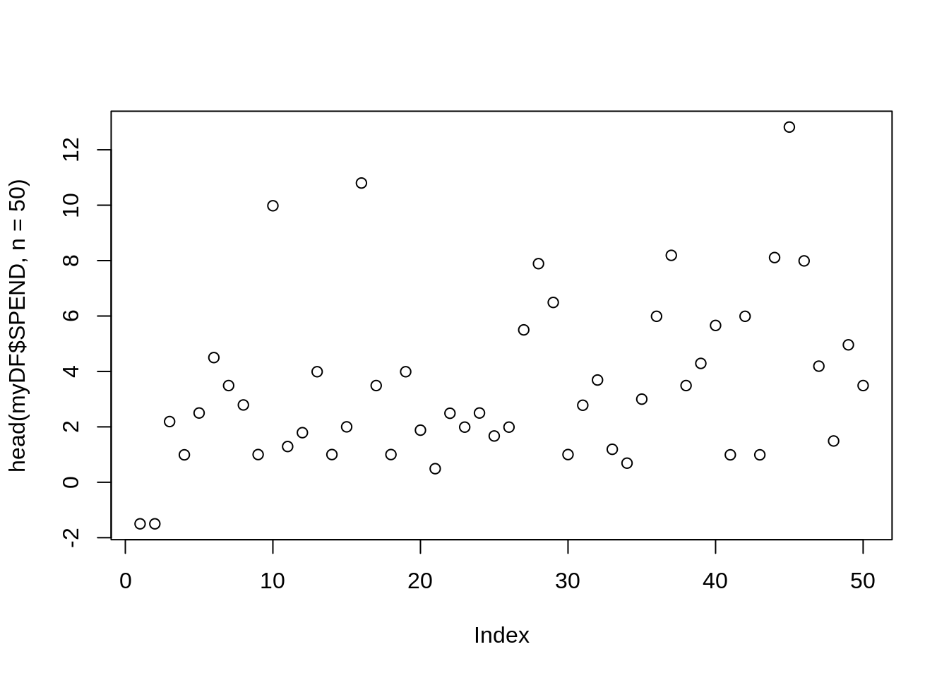
If the result says Error in plot.new() : figure margins too large then you just need to make your plotting window a little bigger, so that R has room to make the plot, and then run the line again.
There are 10625553 entries in the SPEND column:
length(myDF$SPEND)## [1] 1000000This makes sense, because the data frame has 10625553 rows and 9 columns.
dim(myDF)## [1] 1000000 9There are 6322739 entries larger than 2.
length(myDF$SPEND[myDF$SPEND > 2])## [1] 593322There are 451155 entries larger than 10.
length(myDF$SPEND[myDF$SPEND > 10])## [1] 42202There are 4197 entries less than -3.
length(myDF$SPEND[myDF$SPEND <= -3])## [1] 420We encourage you to play with the data sets, and to learn how to work with the data, by trying things yourself, and by asking questions. We always welcome your questions, and we love for you to post questions on Piazza. This is a great way for the entire community to learn together!
Examples using the New York City yellow taxi cab data set.
Please see https://piazza.com/class/kdrxb6dxa8c6by?cid=110 for example code, to go along with this video.
This data set contains the information about the yellow taxi cab rides in New York City in June 2019.
myDF <- read.csv("/class/datamine/data/taxi/yellow/yellow_tripdata_2019-06.csv")Here is the information about the first 6 taxi cab rides. You need to imagine that your computer monitor is much, much wider than it actually is, so that your data has room to stretch out in 6 rows across your screen. Instead, right now, the data wraps around, a few columns at a time. This is probably obvious when you look at it. Each column has a column header.
head(myDF)## VendorID tpep_pickup_datetime tpep_dropoff_datetime passenger_count
## 1 1 2019-06-01 00:55:13 2019-06-01 00:56:17 1
## 2 1 2019-06-01 00:06:31 2019-06-01 00:06:52 1
## 3 1 2019-06-01 00:17:05 2019-06-01 00:36:38 1
## 4 1 2019-06-01 00:59:02 2019-06-01 00:59:12 0
## 5 1 2019-06-01 00:03:25 2019-06-01 00:15:42 1
## 6 1 2019-06-01 00:28:31 2019-06-01 00:39:23 2
## trip_distance RatecodeID store_and_fwd_flag PULocationID DOLocationID
## 1 0.0 1 N 145 145
## 2 0.0 1 N 262 263
## 3 4.4 1 N 74 7
## 4 0.8 1 N 145 145
## 5 1.7 1 N 113 148
## 6 1.6 1 N 79 125
## payment_type fare_amount extra mta_tax tip_amount tolls_amount
## 1 2 3.0 0.5 0.5 0.00 0
## 2 2 2.5 3.0 0.5 0.00 0
## 3 2 17.5 0.5 0.5 0.00 0
## 4 2 2.5 1.0 0.5 0.00 0
## 5 1 9.5 3.0 0.5 2.65 0
## 6 1 9.5 3.0 0.5 1.00 0
## improvement_surcharge total_amount congestion_surcharge
## 1 0.3 4.30 0.0
## 2 0.3 6.30 2.5
## 3 0.3 18.80 0.0
## 4 0.3 4.30 0.0
## 5 0.3 15.95 2.5
## 6 0.3 14.30 2.5The mean cost (i.e., the average cost) of a taxi cab ride in New York City in June 2019 is 19.74, i.e., almost 20 dollars.
mean(myDF$total_amount)## [1] 19.33511The mean number of passengers in a taxi cab ride is 1.567322.
mean(myDF$passenger_count)## [1] 1.567329We can use the table function to tabulate the results of the number of taxi cab rides, according to the passenger_count
For instance, in this case, there are 128130 taxi cab rides with 0 passengers, there are 4854651 taxi cab rides with 1 passenger, there are 1061648 taxi cab rides with 2 passengers, etc.
table(myDF$passenger_count)##
## 0 1 2 3 4 5 6 7 8 9
## 19336 697349 154878 43720 20051 39156 25497 8 3 2We can look at each passenger_count for which the passenger_count equals 4. Of course, the results are all just the value 4!
head(myDF$passenger_count[myDF$passenger_count == 4])## [1] 4 4 4 4 4 4On a more interesting note, we can look at the total cost of a taxi cab ride with 4 passengers. The first 6 rides that (each) have 4 passengers have these 6 costs:
head(myDF$total_amount[myDF$passenger_count == 4])## [1] 8.30 16.80 14.80 9.95 10.30 37.56The average cost of a taxi cab ride with 4 passengers is 20.42111, i.e., just a little more than 20 dollars.
mean(myDF$total_amount[myDF$passenger_count == 4])## [1] 19.73445Altogether, our data set has 6941024 rows and 18 columns.
dim(myDF)## [1] 1000000 18For this reason, the total_amount column has 6941024 entries.
length(myDF$total_amount)## [1] 1000000The amounts of the first 6 taxi cab rides are:
head(myDF$total_amount)## [1] 4.30 6.30 18.80 4.30 15.95 14.30These are the amounts of the first 6 taxi cab rides that each cost more than 100 dollars.
head(myDF$total_amount[myDF$total_amount > 100])## [1] 104.30 120.80 158.90 181.30 112.35 116.30There are 16681 taxi cab rides that (each) cost more than 100 dollars.
length(myDF$total_amount[myDF$total_amount > 100])## [1] 2180If we only include the taxi cab rides that (each) cost more than 100 dollars, the average number of passengers is 1.545051.
mean(myDF$passenger_count[myDF$total_amount > 100])## [1] 1.563303There are 6941024 taxi cab rides altogether.
length(myDF$passenger_count)## [1] 1000000If we ask for the length of the taxi cab rides with total_amount > 100, we might expect to get a smaller number, but again we get 6941024.
length(myDF$total_amount > 100)## [1] 1000000This might be confusing at first, but we can look at the head of those results. This is a vector of 6941024 occurrences of TRUE and FALSE, one per taxi cab ride.
head(myDF$total_amount > 100)## [1] FALSE FALSE FALSE FALSE FALSE FALSEThe way to find out that there are only 16681 taxi cab rides that cost more than 100 dollars is (as we did before) to use the TRUE values as an index into another vector, like this:
length(myDF$total_amount[myDF$total_amount > 100])## [1] 2180or like this
sum(myDF$total_amount > 100)## [1] 2180In this latter method, we turn the TRUE values into 1's and the FALSE values into 0's (this happens automatically when we sum them up) and so we have 16681 values of 1's and the rest are 0's so the sum is 16681, just like we saw above.
Variables
NA
NA stands for not available and, in general, represents a missing value or a lack of data.
How do I tell if a value is NA?
Click here for solution
# Test if value is NA.
value <- NA
is.na(value)
## [1] TRUE# Does is.nan return TRUE for NA?
is.nan(value)## [1] FALSENaN
NaN stands for not a number and, in general, is used for arithmetic purposes, for example, the result of 0/0.
How do I tell if a value is NaN?
Click here for solution
# Test if a value is NaN.
value <- NaN
is.nan(value)
## [1] TRUEvalue <- 0/0
is.nan(value)## [1] TRUE# Does is.na return TRUE for NaN?
is.na(value)## [1] TRUENULL
NULL represents the null object, and is often returned when we have undefined values.
How do I tell if a value is NULL?
Click here for solution
# Test if a value is NaN.
value <- NULL
is.null(value)
## [1] TRUEclass(value)## [1] "NULL"# Does is.na return TRUE for NULL?
is.na(value)## logical(0)Dates
Date is a class which allows you to perform special operations like subtraction, where the number of days between dates are returned. Or addition, where you can add 30 to a Date and a Date is returned where the value is 30 days in the future.
You will usually need to specify the format argument based on the format of your date strings. For example, if you had a string 07/05/1990, the format would be: %m/%d/%Y. If your string was 31-12-90, the format would be %d-%m-%y. Replace %d, %m, %Y, and %y according to your date strings. A full list of formats can be found here.
How do I convert a string "07/05/1990" to a Date?
Click here for solution
my_string <- "07/05/1990"
my_date <- as.Date(my_string, format="%m/%d/%Y")
my_date
## [1] "1990-07-05"How do I convert a string "31-12-1990" to a Date?
Click here for solution
my_string <- "31-12-1990"
my_date <- as.Date(my_string, format="%d-%m-%Y")
my_date
## [1] "1990-12-31"How do I convert a string "12-31-1990" to a Date?
Click here for solution
my_string <- "12-31-1990"
my_date <- as.Date(my_string, format="%m-%d-%Y")
my_date
## [1] "1990-12-31"How do I convert a string "31121990" to a Date?
Click here for solution
my_string <- "31121990"
my_date <- as.Date(my_string, format="%d%m%Y")
my_date
## [1] "1990-12-31"Factors
A factor is R's way of representing a categorical variable. There are entries in a factor (just like there are entries in a vector), but they are constrained to only be chosen from a specific set of values, called the levels of the factor. They are useful when a vector has only a few different values it could be, like "Male" and "Female" or "A", "B", or "C".
How do I test whether or not a vector is a factor?
Click here for solution
test_factor <- factor("Male")
is.factor(test_factor)
## [1] TRUEtest_factor_vec <- factor(c("Male", "Female", "Female"))
is.factor(test_factor_vec)## [1] TRUEHow do I convert a vector of strings to a factor?
Click here for solution
vec <- c("Male", "Female", "Female")
vec <- factor(c("Male", "Female", "Female"))
How do I get the unique values a factor could hold, also known as levels?
Click here for solution
vec <- factor(c("Male", "Female", "Female"))
levels(vec)
## [1] "Female" "Male"How can I rename the levels of a factor?
Click here for solution
vec <- factor(c("Male", "Female", "Female"))
levels(vec)
## [1] "Female" "Male"levels(vec) <- c("F", "M")
vec## [1] M F F
## Levels: F M# Be careful! Order matters, this is wrong:
vec <- factor(c("Male", "Female", "Female"))
levels(vec)## [1] "Female" "Male"levels(vec) <- c("M", "F")
vec## [1] F M M
## Levels: M FHow can I find the number of levels of a factor?
Click here for solution
vec <- factor(c("Male", "Female", "Female"))
nlevels(vec)
## [1] 2Logical operators
Logical operators are symbols that can be used within R to compare values or vectors of values.
| Operator | Description |
|---|---|
< |
less than |
<= |
less than or equal to |
> |
greater than |
>= |
greater than or equal to |
== |
equal to |
!= |
not equal to |
!x |
negation, not x |
x|y |
x OR y |
x&y |
x AND y |
Examples
What are the values in a vector, vec that are greater than 5?
Click here for solution
vec <- 1:10
vec > 5
## [1] FALSE FALSE FALSE FALSE FALSE TRUE TRUE TRUE TRUE TRUEWhat are the values in a vector, vec that are greater than or equal to 5?
Click here for solution
vec <- 1:10
vec >= 5
## [1] FALSE FALSE FALSE FALSE TRUE TRUE TRUE TRUE TRUE TRUEWhat are the values in a vector, vec that are less than 5?
Click here for solution
vec <- 1:10
vec < 5
## [1] TRUE TRUE TRUE TRUE FALSE FALSE FALSE FALSE FALSE FALSEWhat are the values in a vector, vec that are less than or equal to 5?
Click here for solution
vec <- 1:10
vec <= 5
## [1] TRUE TRUE TRUE TRUE TRUE FALSE FALSE FALSE FALSE FALSEWhat are the values in a vector that are greater than 7 OR less than or equal to 2?
Click here for solution
vec <- 1:10
vec > 7 | vec <=2
## [1] TRUE TRUE FALSE FALSE FALSE FALSE FALSE TRUE TRUE TRUEWhat are the values in a vector that are greater than 3 AND less than 6?
Click here for solution
vec <- 1:10
vec > 3 & vec < 6
## [1] FALSE FALSE FALSE TRUE TRUE FALSE FALSE FALSE FALSE FALSEHow do I get the values in list1 that are in list2?
Click here for solution
list1 <- c("this", "is", "a", "test")
list2 <- c("this", "a", "exam")
list1[list1 %in% list2]
## [1] "this" "a"How do I get the values in list1 that are not in list2?
Click here for solution
list1 <- c("this", "is", "a", "test")
list2 <- c("this", "a", "exam")
list1[!(list1 %in% list2)]
## [1] "is" "test"How can I get the number of values in a vector that are greater than 5?
Click here for solution
vec <- 1:10
sum(vec>5)
## [1] 5# Note, you do not need to do:
length(vec[vec>5])## [1] 5# because TRUE==1 and FALSE==0 in R
TRUE==1## [1] TRUEFALSE==0## [1] TRUELists & Vectors
A vector contains values that are all the same type. The following are some examples of vectors:
# A logical vector
lvec <- c(F, T, TRUE, FALSE)
class(lvec)
## [1] "logical"# A numeric vector
nvec <- c(1,2,3,4)
class(nvec)## [1] "numeric"# A character vector
cvec <- c("this", "is", "a", "test")
class(cvec)## [1] "character"As soon as you try to mix and match types, elements are coerced to the simplest type required to represent all the data.
The order of representation is:
logical, numeric, character, list
For example:
class(c(F, 1, 2))## [1] "numeric"class(c(F, 1, 2, "ok"))## [1] "character"class(c(F, 1, 2, "ok", list(1, 2, "ok")))## [1] "list"Lists are vectors that can contain any class of data. For example:
list(TRUE, 1, 2, "OK", c(1,2,3))## [[1]]
## [1] TRUE
##
## [[2]]
## [1] 1
##
## [[3]]
## [1] 2
##
## [[4]]
## [1] "OK"
##
## [[5]]
## [1] 1 2 3With lists, there are 3 ways you can index.
my_list <- list(TRUE, 1, 2, "OK", c(1,2,3), list("OK", 1,2, F))

# The first way is with single square brackets [].
# This will always return a list, even if the content
# only has 1 component.
class(my_list[1:2])
## [1] "list"class(my_list[3])## [1] "list"# The second way is with double brackets [[]].
# This will return the content itself. If the
# content is something other than a list it will
# return the value itself.
class(my_list[[1]])## [1] "logical"class(my_list[[3]])## [1] "numeric"# Of course, if the value is a list itself, it will
# remain a list.
class(my_list[[6]])## [1] "list"# The third way is using $ to extract a single, named variable.
# We need to add names first! $ is like the double bracket,
# in that it will return the simplest form.
my_list <- list(first=TRUE, second=1, third=2, fourth="OK", embedded_vector=c(1,2,3), embedded_list=list("OK", 1,2, F))
my_list$first## [1] TRUEmy_list$embedded_list## [[1]]
## [1] "OK"
##
## [[2]]
## [1] 1
##
## [[3]]
## [1] 2
##
## [[4]]
## [1] FALSEHow do get the type of a vector?
Click here for solution
my_vector <- c(0, 1, 2)
typeof(my_vector)
## [1] "double"How do I convert a character vector to a numeric?
Click here for solution
my_character_vector <- c('1','2','3','4')
as.numeric(my_character_vector)
## [1] 1 2 3 4How do I convert a numeric vector to a character?
Click here for solution
my_numeric_vector <- c(1,2,3,4)
as.character(my_numeric_vector)
## [1] "1" "2" "3" "4"Indexing
Indexing enables us to access a subset of the elements in vectors and lists. There are three types of indexing: positional/numeric, logical, and reference/named.
You can create a named vector and a named list easily:
my_vec <- 1:5
names(my_vec) <- c("alpha","bravo","charlie","delta","echo")

my_list <- list(1,2,3,4,5)
names(my_list) <- c("alpha","bravo","charlie","delta","echo")

my_list2 <- list("alpha" = 1, "beta" = 2, "charlie" = 3, "delta" = 4, "echo" = 5)
# Numeric (positional) indexing:
my_vec[1:2]## alpha bravo
## 1 2my_vec[c(1,3)]## alpha charlie
## 1 3my_list[1:2]## $alpha
## [1] 1
##
## $bravo
## [1] 2my_list[c(1,3)]## $alpha
## [1] 1
##
## $charlie
## [1] 3# Logical indexing:
my_vec[c(T, F, T, F, F)]## alpha charlie
## 1 3my_list[c(T, F, T, F, F)]## $alpha
## [1] 1
##
## $charlie
## [1] 3# Named (reference) indexing:
# if there are named values:
my_vec[c("alpha", "charlie")]## alpha charlie
## 1 3my_list[c("alpha", "charlie")]## $alpha
## [1] 1
##
## $charlie
## [1] 3In addition, you can use negative indexing. Negative indexing works differently than in Python where the index starts at the end instead of the beginning. In R, a negative index removes the index from the output. For example:
my_vec[-2]## alpha charlie delta echo
## 1 3 4 5You can pass multiple values as well:
my_vec[-c(2,3)]## alpha delta echo
## 1 4 5Examples
How can I get the first 2 values of a vector named my_vec?
Click here for solution
my_vec <- c(1, 13, 2, 9)
names(my_vec) <- c('cat', 'dog','snake', 'otter')
my_vec[1:2]
## cat dog
## 1 13How can I get the values that are greater than 2?
Click here for solution
my_vec[my_vec>2]## dog otter
## 13 9How can I get the values greater than 5 and smaller than 10?
Click here for solution
my_vec[my_vec > 5 & my_vec < 10]## otter
## 9How can I get the values greater than 10 or smaller than 3?
Click here for solution
my_vec[my_vec > 10 | my_vec < 3]## cat dog snake
## 1 13 2How can I get the values for "otter" and "dog"?
Click here for solution
my_vec[c('otter','dog')]## otter dog
## 9 13Recycling
Often operations in R on two or more vectors require them to be the same length. When R encounters vectors with different lengths, it automatically repeats (recycles) the shorter vector until the length of the vectors is the same.
Examples
Given two numeric vectors with different lengths, add them element-wise.
Click here for solution
x <- c(1,2,3)
y <- c(0,1)
x+y
## Warning in x + y: longer object length is not a multiple of shorter object
## length## [1] 1 3 3Basic R functions
all
all returns a logical value (TRUE or FALSE) if all values in a vector are TRUE.
Examples
Are all values in x positive?
Click here for solution
x <- c(1, 2, 3, 4, 8, -1, 7, 3, 4, -2, 1, 3)
all(x>0) # FALSE
## [1] FALSEany
any returns a logical value (TRUE or FALSE) if any values in a vector are TRUE.
Examples
Are any values in x positive?
Click here for solution
x <- c(1, 2, 3, 4, 8, -1, 7, 3, 4, -2, 1, 3)
any(x>0) # TRUE
## [1] TRUEall.equal
all.equal compares two objects and tests if they are "nearly equal" (up to some provided tolerance).
Examples
Is \(\pi\) equal to 3.14?
Click here for solution
all.equal(pi, 3.14) # FALSE## [1] "Mean relative difference: 0.0005069574"Is \(\pi\) equal to 3.14 if our tolerance is 2 decimal cases?
Click here for solution
all.equal(pi, 3.14, tol=0.01) # TRUE## [1] TRUEAre the vectors x and y equal?
Click here for solution
x <- 1:5
y <- c('1', '2', '3', '4', '5')
all.equal(x, y) # difference in type (numeric vs. character)
## [1] "Modes: numeric, character"
## [2] "target is numeric, current is character"all.equal(x, as.numeric(y)) # TRUE## [1] TRUE%in%
Although %in% doesn't look like it, it is a function. Given two vectors, %in% returns a logical vector indicating if the respective values in the left operand have a match in the right operand.
You can learn more about %in% by running ?"%in%".
Examples
How do I find whether or not a value, 5 is in a given vector?
Click here for solution
5 %in% c(1,2,3)## [1] FALSE5 %in% c(3,4,5)## [1] TRUEHow can I find which values in one vector are present in another?
Click here for solution
c(1,2,3) %in% c(1,2)c(1,2,3) %in% c(3,4,5)
# order doesn't matter for the right operand
c(1,2,3) %in% c(5,3,4)setdiff
Given two vectors, the function setdiff returns the element of the first vector which do not exist in the second vector. Note: The order in which the vectors are listed in relation to the function setdiff matters, as illustrated in the first two examples.
Examples
Let x = (a, b, b, c) and y = (c, b, d, e, f). How to I find the elements in vector x that are not in vector y?
Click here for solution
x <- c('a','b','b','c')
y <- c('c','b','d','e','f')
setdiff(x,y)
## [1] "a"setdiff(y,x)## [1] "d" "e" "f"How to I find the elements in vector y that are not in vector x?
Click here for solution
x <- c('a','b','b','c')
y <- c('c','b','d','e','f')
setdiff(y,x)
## [1] "d" "e" "f"intersect
The intersect function returns the elements that two vectors or data.frames have in common.
Note: The order in which the vectors are listed in relation to the function intersect only affects the order of the common elements returned.
Examples
dim
dim returns the dimensions of a matrix or data.frame. The first value is the rows, the second is columns.
Examples
How many dimensions does the data.frame dat have?
Click here for solution
dat <- data.frame("col1"=c(1,2,3), "col2"=c("a", "b", "c"))
dim(dat) # 3 rows and 2 columns
## [1] 3 2length
length allows you to get or set the length of an object in R (for which a method has been defined).
How do I get how many values are in a vector?
Click here for solution
# Create a vector of length 5
my_vector <- c(1,2,3,4,5)

# Calculate the length of my_vector
length(my_vector)
## [1] 5rep
rep is short for replicate. rep accepts some object, x, and up to three additional arguments: times, length.out, and each. times is the number of non-negative times to repeat the whole object x. length.out specifies the end length you want the result to be. rep will repeat the values in x as many times as it takes to reach the provided length.out. each repeats each element in x the number of times specified by each.
Examples
How do I repeat values in a vector 3 times?
Click here for solution
vec <- c(1,2,3)
rep(vec, 3)
## [1] 1 2 3 1 2 3 1 2 3# or
rep(vec, times=3)## [1] 1 2 3 1 2 3 1 2 3How do I repeat the values in a vector enough times to be the same length as another vector?
Click here for solution
vec <- c(1,2,3)
other_vec <- c(1,2,2,2,2,2,2,8)
rep(vec, length.out=length(other_vec))
## [1] 1 2 3 1 2 3 1 2# Note that if the end goal is to do something
# like add the two vectors, this can be done
# using recycling.
rep(vec, length.out=length(other_vec)) + other_vec## [1] 2 4 5 3 4 5 3 10vec + other_vec## Warning in vec + other_vec: longer object length is not a multiple of shorter
## object length## [1] 2 4 5 3 4 5 3 10How can I repeat each value inside a vector a certain amount of times?
Click here for solution
vec <- c(1,2,3)
rep(vec, each=3)
## [1] 1 1 1 2 2 2 3 3 3How can I repeat the values in one vector based on the values in another vector?
Click here for solution
vec <- c(1,2,3)
rep_by <- c(3,2,1)
rep(vec, times=rep_by)
## [1] 1 1 1 2 2 3rbind and cbind
rbind and cbind append objects (vectors, matrices or data.frames) as rows (rbind) or as columns (cbind).
Examples
How do I combine 3 vectors into a matrix?
Click here for solution
x <- 1:10
y <- 11:20
z <- 10:1

# combining them as rows
rbind(x,y,z)
## [,1] [,2] [,3] [,4] [,5] [,6] [,7] [,8] [,9] [,10]
## x 1 2 3 4 5 6 7 8 9 10
## y 11 12 13 14 15 16 17 18 19 20
## z 10 9 8 7 6 5 4 3 2 1dim(rbind(x,y,z))## [1] 3 10# combining them as columns
cbind(x,y,z)## x y z
## [1,] 1 11 10
## [2,] 2 12 9
## [3,] 3 13 8
## [4,] 4 14 7
## [5,] 5 15 6
## [6,] 6 16 5
## [7,] 7 17 4
## [8,] 8 18 3
## [9,] 9 19 2
## [10,] 10 20 1dim(cbind(x,y,z))## [1] 10 3How do I add a vector as a column to a matrix?
Click here for solution
x <- 1:10
my_mat <- matrix(1:20, ncol=2)

my_mat <- cbind(my_mat, x)
dim(my_mat)
## [1] 10 3How do I append new rows to a matrix?
Click here for solution
my_mat1 <- matrix(20:1, ncol=2)
my_mat2 <- matrix(1:20, ncol=2)

my_mat <- rbind(my_mat1, my_mat2)
dim(my_mat)
## [1] 20 2which, which.max, which.min
which enables you to find the position of the elements that are TRUE in a logical vector.
which.max and which.min finds the location of the maximum and minimum, respectively, of a numeric (or logical) vector.
Examples
Given a numeric vector, return the index of the maximum value.
Click here for solution
x <- c(1,-10, 2,4,-3,9,2,-2,4,8)
which.max(x)
## [1] 6# which.max is just shorthand for:
which(x==max(x))## [1] 6Given a vector, return the index of the positive values.
Click here for solution
x <- c(1,-10, 2,4,-3,9,2,-2,4,8)
which(x>0)
## [1] 1 3 4 6 7 9 10Given a matrix, return the indexes (row and column) of the positive values.
Click here for solution
x <- matrix(c(1,-10, 2,4,-3,9,2,-2,4,8), ncol=2)
which(x>0, arr.ind = TRUE)
## row col
## [1,] 1 1
## [2,] 3 1
## [3,] 4 1
## [4,] 1 2
## [5,] 2 2
## [6,] 4 2
## [7,] 5 2grep, grepl, etc.
grep allows you to use regular expressions to search for a pattern in a string or character vector, and returns the index where there is a match.
grepl performs the same operation but rather than returning indices, returns a vector of logical TRUE or FALSE values.
Examples
Given a character vector, return the index of any words ending in "s".
Click here for solution
grep(".*s$", c("waffle", "waffles", "pancake", "pancakes"))## [1] 2 4Given a character vector, return a vector of the same length where each element is TRUE if there was a match for any word ending in "s", and `FALSE otherwise.
Click here for solution
grepl(".*s$", c("waffle", "waffles", "pancake", "pancakes"))## [1] FALSE TRUE FALSE TRUEResources
An excellent quick reference for regular expressions. Examples using grep in R.
sum
sum is a function that calculates the sum of a vector of values.
Examples
How do I get the sum of the values in a vector?
Click here for solution
sum(c(1,3,2,10,4))## [1] 20How do I get the sum of the values in a vector when some of the values are: NA, NaN?
Click here for solution
sum(c(1,2,3,NaN), na.rm=T)## [1] 6sum(c(1,2,3,NA), na.rm=T)## [1] 6sum(c(1,2,NA,NaN,4), na.rm=T)## [1] 7mean
mean is a function that calculates the average of a vector of values.
How do I get the average of a vector of values?
Click here for solution
mean(c(1,2,3,4))## [1] 2.5How do I get the average of a vector of values when some of the values are: NA, NaN?
Click here for solution
Many R functions have the na.rm argument available. This argument is "a logical value indicating whether NA values should be stripped before the computation proceeds."
mean(c(1,2,3,NaN), na.rm=T)## [1] 2mean(c(1,2,3,NA), na.rm=T)## [1] 2mean(c(1,2,NA,NaN,4), na.rm=T)## [1] 2.333333var
var is a function that calculate the variance of a vector of values.
How do I get the variance of a vector of values?
Click here for solution
var(c(1,2,3,4))## [1] 1.666667How do I get the variance of a vector of values when some of the values are: NA, NaN?
Click here for solution
var(c(1,2,3,NaN), na.rm=T)## [1] 1var(c(1,2,3,NA), na.rm=T)## [1] 1var(c(1,2,NA,NaN,4), na.rm=T)## [1] 2.333333How do I get the standard deviation of a vector of values?
Click here for solution
The standard deviation is equal to the square root of the variance.
sqrt(var(c(1,2,3,NaN), na.rm=T))## [1] 1sqrt(var(c(1,2,3,NA), na.rm=T))## [1] 1sqrt(var(c(1,2,NA,NaN,4), na.rm=T))## [1] 1.527525colSums and rowSums
colSums and rowSums calculates row and column sums for numeric matrices or data.frames.
Examples
How do I get the sum of the values for every column in a data frame?
Click here for solution
# First 6 values in mtcars
head(mtcars)
## mpg cyl disp hp drat wt qsec vs am gear carb
## Mazda RX4 21.0 6 160 110 3.90 2.620 16.46 0 1 4 4
## Mazda RX4 Wag 21.0 6 160 110 3.90 2.875 17.02 0 1 4 4
## Datsun 710 22.8 4 108 93 3.85 2.320 18.61 1 1 4 1
## Hornet 4 Drive 21.4 6 258 110 3.08 3.215 19.44 1 0 3 1
## Hornet Sportabout 18.7 8 360 175 3.15 3.440 17.02 0 0 3 2
## Valiant 18.1 6 225 105 2.76 3.460 20.22 1 0 3 1# For every column, sum of all rows:
colSums(mtcars)## mpg cyl disp hp drat wt qsec vs
## 642.900 198.000 7383.100 4694.000 115.090 102.952 571.160 14.000
## am gear carb
## 13.000 118.000 90.000How do I get the sum of the values for every row in a data frame?
Click here for solution
# First 6 values in mtcars
head(mtcars)
## mpg cyl disp hp drat wt qsec vs am gear carb
## Mazda RX4 21.0 6 160 110 3.90 2.620 16.46 0 1 4 4
## Mazda RX4 Wag 21.0 6 160 110 3.90 2.875 17.02 0 1 4 4
## Datsun 710 22.8 4 108 93 3.85 2.320 18.61 1 1 4 1
## Hornet 4 Drive 21.4 6 258 110 3.08 3.215 19.44 1 0 3 1
## Hornet Sportabout 18.7 8 360 175 3.15 3.440 17.02 0 0 3 2
## Valiant 18.1 6 225 105 2.76 3.460 20.22 1 0 3 1# For every row, sum of all columns:
rowSums(mtcars)## Mazda RX4 Mazda RX4 Wag Datsun 710 Hornet 4 Drive
## 328.980 329.795 259.580 426.135
## Hornet Sportabout Valiant Duster 360 Merc 240D
## 590.310 385.540 656.920 270.980
## Merc 230 Merc 280 Merc 280C Merc 450SE
## 299.570 350.460 349.660 510.740
## Merc 450SL Merc 450SLC Cadillac Fleetwood Lincoln Continental
## 511.500 509.850 728.560 726.644
## Chrysler Imperial Fiat 128 Honda Civic Toyota Corolla
## 725.695 213.850 195.165 206.955
## Toyota Corona Dodge Challenger AMC Javelin Camaro Z28
## 273.775 519.650 506.085 646.280
## Pontiac Firebird Fiat X1-9 Porsche 914-2 Lotus Europa
## 631.175 208.215 272.570 273.683
## Ford Pantera L Ferrari Dino Maserati Bora Volvo 142E
## 670.690 379.590 694.710 288.890colMeans and rowMeans
colMeans and rowMeans calculates row and column means for numeric matrices or data.frames.
Examples
Examples
How do I get the mean for every column in a data frame?
Click here for solution
# First 6 values in mtcars
head(mtcars)
## mpg cyl disp hp drat wt qsec vs am gear carb
## Mazda RX4 21.0 6 160 110 3.90 2.620 16.46 0 1 4 4
## Mazda RX4 Wag 21.0 6 160 110 3.90 2.875 17.02 0 1 4 4
## Datsun 710 22.8 4 108 93 3.85 2.320 18.61 1 1 4 1
## Hornet 4 Drive 21.4 6 258 110 3.08 3.215 19.44 1 0 3 1
## Hornet Sportabout 18.7 8 360 175 3.15 3.440 17.02 0 0 3 2
## Valiant 18.1 6 225 105 2.76 3.460 20.22 1 0 3 1# Mean of each column
colMeans(mtcars)## mpg cyl disp hp drat wt qsec
## 20.090625 6.187500 230.721875 146.687500 3.596563 3.217250 17.848750
## vs am gear carb
## 0.437500 0.406250 3.687500 2.812500How do I get the mean for every row in a data frame?
Click here for solution
# First 6 values in mtcars
head(mtcars)
## mpg cyl disp hp drat wt qsec vs am gear carb
## Mazda RX4 21.0 6 160 110 3.90 2.620 16.46 0 1 4 4
## Mazda RX4 Wag 21.0 6 160 110 3.90 2.875 17.02 0 1 4 4
## Datsun 710 22.8 4 108 93 3.85 2.320 18.61 1 1 4 1
## Hornet 4 Drive 21.4 6 258 110 3.08 3.215 19.44 1 0 3 1
## Hornet Sportabout 18.7 8 360 175 3.15 3.440 17.02 0 0 3 2
## Valiant 18.1 6 225 105 2.76 3.460 20.22 1 0 3 1# Mean of each row
rowMeans(mtcars)## Mazda RX4 Mazda RX4 Wag Datsun 710 Hornet 4 Drive
## 29.90727 29.98136 23.59818 38.73955
## Hornet Sportabout Valiant Duster 360 Merc 240D
## 53.66455 35.04909 59.72000 24.63455
## Merc 230 Merc 280 Merc 280C Merc 450SE
## 27.23364 31.86000 31.78727 46.43091
## Merc 450SL Merc 450SLC Cadillac Fleetwood Lincoln Continental
## 46.50000 46.35000 66.23273 66.05855
## Chrysler Imperial Fiat 128 Honda Civic Toyota Corolla
## 65.97227 19.44091 17.74227 18.81409
## Toyota Corona Dodge Challenger AMC Javelin Camaro Z28
## 24.88864 47.24091 46.00773 58.75273
## Pontiac Firebird Fiat X1-9 Porsche 914-2 Lotus Europa
## 57.37955 18.92864 24.77909 24.88027
## Ford Pantera L Ferrari Dino Maserati Bora Volvo 142E
## 60.97182 34.50818 63.15545 26.26273unique
unique "returns a vector, data frame, or array like x but with duplicate elements/rows removed.
Given a vector of values, how do I return a vector of values with all duplicates removed?
Click here for solution
vec <- c(1, 2, 3, 3, 3, 4, 5, 5, 6)
unique(vec)
## [1] 1 2 3 4 5 6summary
summary shows summary statistics for a vector, or for every column in a data.frame and/or matrix. The summary statistics shown are: mininum value, maximum value, first and third quartiles, mean and median.
Examples
How do I get summary statistics for a vector?
Click here for solution
summary(1:30)## Min. 1st Qu. Median Mean 3rd Qu. Max.
## 1.00 8.25 15.50 15.50 22.75 30.00How do I get summary statistics for every column in a data frame?
Click here for solution
# First 6 values in mtcars
head(mtcars)
## mpg cyl disp hp drat wt qsec vs am gear carb
## Mazda RX4 21.0 6 160 110 3.90 2.620 16.46 0 1 4 4
## Mazda RX4 Wag 21.0 6 160 110 3.90 2.875 17.02 0 1 4 4
## Datsun 710 22.8 4 108 93 3.85 2.320 18.61 1 1 4 1
## Hornet 4 Drive 21.4 6 258 110 3.08 3.215 19.44 1 0 3 1
## Hornet Sportabout 18.7 8 360 175 3.15 3.440 17.02 0 0 3 2
## Valiant 18.1 6 225 105 2.76 3.460 20.22 1 0 3 1# Mean of each column
summary(mtcars)## mpg cyl disp hp
## Min. :10.40 Min. :4.000 Min. : 71.1 Min. : 52.0
## 1st Qu.:15.43 1st Qu.:4.000 1st Qu.:120.8 1st Qu.: 96.5
## Median :19.20 Median :6.000 Median :196.3 Median :123.0
## Mean :20.09 Mean :6.188 Mean :230.7 Mean :146.7
## 3rd Qu.:22.80 3rd Qu.:8.000 3rd Qu.:326.0 3rd Qu.:180.0
## Max. :33.90 Max. :8.000 Max. :472.0 Max. :335.0
## drat wt qsec vs
## Min. :2.760 Min. :1.513 Min. :14.50 Min. :0.0000
## 1st Qu.:3.080 1st Qu.:2.581 1st Qu.:16.89 1st Qu.:0.0000
## Median :3.695 Median :3.325 Median :17.71 Median :0.0000
## Mean :3.597 Mean :3.217 Mean :17.85 Mean :0.4375
## 3rd Qu.:3.920 3rd Qu.:3.610 3rd Qu.:18.90 3rd Qu.:1.0000
## Max. :4.930 Max. :5.424 Max. :22.90 Max. :1.0000
## am gear carb
## Min. :0.0000 Min. :3.000 Min. :1.000
## 1st Qu.:0.0000 1st Qu.:3.000 1st Qu.:2.000
## Median :0.0000 Median :4.000 Median :2.000
## Mean :0.4062 Mean :3.688 Mean :2.812
## 3rd Qu.:1.0000 3rd Qu.:4.000 3rd Qu.:4.000
## Max. :1.0000 Max. :5.000 Max. :8.000order and sort
sort allows you to arrange (or partially arrange) a vector into ascending or descending order.
order returns the position of each element of a vector in ascending (or descending order).
Examples
Given a vector, arrange it in a ascending order.
Click here for solution
x <- c(1,3,2,10,4)
sort(x)
## [1] 1 2 3 4 10Given a vector, arrange it in a descending order.
Click here for solution
x <- c(1,3,2,10,4)
sort(x, decreasing = TRUE)
## [1] 10 4 3 2 1Given a character vector, arrange it in ascending order.
Click here for solution
sort(c("waffle", "pancake", "eggs", "bacon"))## [1] "bacon" "eggs" "pancake" "waffle"Given a matrix, arrange it in ascending order using the first column.
Click here for solution
my_mat <- matrix(c(1,5,0, 2, 10, 1, 2, 8, 9, 1,0,2), ncol=3)
my_mat[order(my_mat[,1]),]
## [,1] [,2] [,3]
## [1,] 0 2 0
## [2,] 1 10 9
## [3,] 2 8 2
## [4,] 5 1 1paste and paste0
paste is a useful function to "concatenate vectors after converting to character."
paste0 is a shorthand function where the sep argument is "".
How do I concatenate two vectors, element-wise, with a comma in between values from each vector?
Click here for solution
vector1 <- c("one", "three", "five")
vector2 <- c("two", "four", "six")
paste(vector1, vector2, sep=",")
## [1] "one,two" "three,four" "five,six"How do I paste together two strings?
Click here for solution
paste0("abra", "kadabra")## [1] "abrakadabra"How do I paste together three strings?
Click here for solution
paste0("abra", "kadabra", "alakazam")## [1] "abrakadabraalakazam"head and tail
head returns the first n (default is 6) parts of a vector, matrix, table, data.frame or function. For vectors, head shows the first 6 values, for matrices, tables and data.frame, head shows the first 6 rows, and for functions the first 6 rows of code.
tail returns the last n (default is 6) parts of a vector, matrix, table, data.frame or function.
Examples
How do I get the first 6 rows of a data.frame?
Click here for solution
head(df)##
## 1 function (x, df1, df2, ncp, log = FALSE)
## 2 {
## 3 if (missing(ncp))
## 4 .Call(C_df, x, df1, df2, log)
## 5 else .Call(C_dnf, x, df1, df2, ncp, log)
## 6 }How do I get the first 10 rows of a data.frame?
Click here for solution
head(df, 10)##
## 1 function (x, df1, df2, ncp, log = FALSE)
## 2 {
## 3 if (missing(ncp))
## 4 .Call(C_df, x, df1, df2, log)
## 5 else .Call(C_dnf, x, df1, df2, ncp, log)
## 6 }How do I get the last 6 rows of a data.frame?
Click here for solution
tail(df)##
## 1 function (x, df1, df2, ncp, log = FALSE)
## 2 {
## 3 if (missing(ncp))
## 4 .Call(C_df, x, df1, df2, log)
## 5 else .Call(C_dnf, x, df1, df2, ncp, log)
## 6 }How do I get the last 8 rows of a data.frame?
Click here for solution
tail(df, 8)##
## 1 function (x, df1, df2, ncp, log = FALSE)
## 2 {
## 3 if (missing(ncp))
## 4 .Call(C_df, x, df1, df2, log)
## 5 else .Call(C_dnf, x, df1, df2, ncp, log)
## 6 }str
str stands for structure. str gives you a glimpse at the variable of interest.
Examples
How do I get the number of columns or features in a data.frame?
Click here for solution
As you can see, there are 9 rows or obs. (short for observations), and 29 variables (which can be referred to as columns or features).
str(df)strsplit
strsplit accepts a vector of strings, and a vector of strings representing regular expressions. Each string in the first vector is split according to the respective string in the second vector.
Examples
How do I split a string containing multiple sentences into individual sentences?
Click here for solution
Note that you need to escape the "." as "." means "any character" in regular expressions. In R, you put two "" before it.
multiple_sentences <- "This is the first sentence. This is the second sentence. This is the third sentence."
unlist(strsplit(multiple_sentences, "\\."))
## [1] "This is the first sentence" " This is the second sentence"
## [3] " This is the third sentence"# remove extra whitespace
trimws(unlist(strsplit(multiple_sentences, "\\.")))## [1] "This is the first sentence" "This is the second sentence"
## [3] "This is the third sentence"How do I split one string by a space, and the next string by a "."?
Click here for solution
string_vec <- c("Okay okay you win.", "This. Is. Not. Okay.")
strsplit(string_vec, c(" ", "\\."))
## [[1]]
## [1] "Okay" "okay" "you" "win."
##
## [[2]]
## [1] "This" " Is" " Not" " Okay"names
names is a function that returns the names of a an object. This includes the typical data structures: vectors, lists, and data.frames. By default, names will return the column names of a data.frame, not the row names.
Examples
How do I get the column names of a data.frame?
Click here for solution
# Get the column names of a data.frame
names(df)
## [1] "cat_1" "cat_2" "ok" "other"How do I get the names of a list?
Click here for solution
# Get the names of a list
names(list(col1=c(1,2,3), col2=c(987)))
## [1] "col1" "col2"How do I get the names of a vector?
Click here for solution
# Get the names of a vector
names(c(val1=1, val2=2, val3=3))
## [1] "val1" "val2" "val3"How do I change the column names of a data.frame?
Click here for solution
names(df) <- c("col1", "col2", "col3", "col4")
df
## col1 col2 col3 col4
## 1 1 9 TRUE first
## 2 2 8 TRUE second
## 3 3 7 FALSE thirdcolnames & rownames
colnames is the same as names but specifies the column names. rownames is the same as names but specifies the row names.
table & prop.table
table is a function used to build a contingency table of counts of various factors.
prop.table is a function that accepts the output of table and rather than returning counts, returns conditional proportions.
Examples
How do I get a count of the number of students in each year in our grades data.frame?
Click here for solution
table(grades$year)##
## freshman junior senior sophomore
## 1 4 2 3How do I get the precentages of students in each year in our grades data.frame?
Click here for solution
prop.table(table(grades$year))##
## freshman junior senior sophomore
## 0.1 0.4 0.2 0.3How do I get a count of the number of students in each year by sex in our grades data.frame?
Click here for solution
table(grades$year, grades$sex)##
## F M
## freshman 0 1
## junior 2 2
## senior 1 1
## sophomore 1 2How do I get the precentages of students in each year by sex in our grades data.frame?
Click here for solution
prop.table(table(grades$year, grades$sex))##
## F M
## freshman 0.0 0.1
## junior 0.2 0.2
## senior 0.1 0.1
## sophomore 0.1 0.2cut
cut breaks a vector x into factors specified by the argument breaks. cut is particularly useful to break Date data into categories like "Q1", "Q2", or 1998, 1999, 2000, etc.
You can find more useful information by running ?cut.POSIXt.
Examples
How can I create a new column in a data.frame df that is a factor based on the year?
Click here for solution
df$year <- cut(df$times, breaks="year")
str(df)
## 'data.frame': 24 obs. of 3 variables:
## $ times: POSIXct, format: "2020-06-01 06:00:00" "2020-07-01 06:00:00" ...
## $ value: int 48 62 55 4 83 77 5 53 68 46 ...
## $ year : Factor w/ 3 levels "2020-01-01","2021-01-01",..: 1 1 1 1 1 1 1 2 2 2 ...How can I create a new column in a data.frame df that is a factor based on the quarter?
Click here for solution
df$quarter <- cut(df$times, breaks="quarter")
str(df)
## 'data.frame': 24 obs. of 4 variables:
## $ times : POSIXct, format: "2020-06-01 06:00:00" "2020-07-01 06:00:00" ...
## $ value : int 48 62 55 4 83 77 5 53 68 46 ...
## $ year : Factor w/ 3 levels "2020-01-01","2021-01-01",..: 1 1 1 1 1 1 1 2 2 2 ...
## $ quarter: Factor w/ 9 levels "2020-04-01","2020-07-01",..: 1 2 2 2 3 3 3 4 4 4 ...How can I create a new column in a data.frame df that is a factor based on every 2 weeks?
Click here for solution
df$biweekly <- cut(df$times, breaks="2 weeks")For an example with the 7581 data set:
myDF <- read.csv("/class/datamine/data/fars/7581.csv")These are the values of the HOUR column:
table(myDF$HOUR)We can break these values into 6-hour intervals:
table( cut(myDF$HOUR, breaks=c(0,6,12,18,24,99), include.lowest=T) )and then find the total number of PERSONS who are involved in accidents during each 6-hour interval
tapply( myDF$PERSONS, cut(myDF$HOUR, breaks=c(0,6,12,18,24,99), include.lowest=T), sum )subset
subset is a function that helps you take subsets of data. By default, subset removes NA rows, so use with care. subset does not perform any operation that can't be accomplished by indexing, but can sometimes be easier to read.
Where we would normally write something like:
grades[grades$year=="junior" | grades$sex=="M",]$grade## [1] 100 75 74 69 88 99 90 92We can instead do:
subset(grades, year=="junior" | sex=="M", select=grade)## grade
## 1 100
## 3 75
## 4 74
## 6 69
## 7 88
## 8 99
## 9 90
## 10 92But be careful, if we replace a grade with an NA, it will be removed by subset:
grades$sex[8] <- NA
subset(grades, year=="junior" | sex=="M", select=grade)
## grade
## 1 100
## 3 75
## 4 74
## 6 69
## 7 88
## 9 90
## 10 92Whereas indexing will not unless you specify to:
grades[grades$year=="junior" | grades$sex=="M",]$grade## [1] 100 75 74 69 88 NA 90 92How can I easily make a subset of the 8451 data, using only 1 line of R, with the subset function?
In the 84.51 data set:
myDF <- read.csv("/class/datamine/data/8451/The_Complete_Journey_2_Master/5000_transactions.csv")We recall that these are the variables:
head(myDF)and there are 10625553 rows and 9 columns
dim(myDF)We can use the subset command to focus on only the purchases from the CENTRAL store region, in the YEAR 2016. We can also pick which variables that we want to have in this new data frame.
Please note: We do not need to specify myDF on each variable, because the subset function will keep track of this for us. The subset function knows which data set that we are working with, because we specify it as the first parameter in the subset function.
The subset parameter of the subset function describes the rows that we are interested in. (In particular, we specify the conditions that we want the rows to satisfy.)
The select parameter of the subset function describes the columns that we are interested in. (We list the columns by their names, and we need to put each such column name in double quotes.)
myfocusedDF <- subset(myDF, subset=(STORE_R=="CENTRAL") & (YEAR==2016),
                            select=c("PURCHASE_","PRODUCT_NUM","SPEND","UNITS") )
This new data set has only 1246144 rows, i.e., about 12 percent of the purchases, as expected. It also has only the 4 columns that we specified in the subset function.
dim(myfocusedDF)How can I easily make a subset of the election data, using only 1 line of R, with the subset function?
Here is an example of how to use the subset function with the data from the federal election campaign contributions from 2016:
library(data.table)
myDF <- fread("/class/datamine/data/election/itcont2016.txt", sep="|")
There were 20557796 donations made in 2016:
dim(myDF)We can use the subset command to focus on the donations made from Midwest states, and limit our results to those donations that had positive TRANSACTION_AMT values. We can extract interesting variables, e.g., the NAME, CITY, STATE, and TRANSACTION_AMT.
mymidwestDF <- subset(myDF, subset=(STATE %in% c("IN","IL","OH","MI","WI")) & (TRANSACTION_AMT > 0),
                      select=c("NAME","CITY","STATE","TRANSACTION_AMT") )
The resulting data frame has 2435825 rows.
dim(mymidwestDF)From the data set, we can sum the TRANSACTION_AMT values, grouped according to the NAME of the donor, and we find that EYCHANER, FRED was the top donor living in the midwest, during the 2016 federal election campaigns.
tail(sort(tapply(mymidwestDF$TRANSACTION_AMT, mymidwestDF$NAME, sum)))difftime {r#-difftime}
The function difftime computes/creates a time interval between two dates/times and converts the interval to a chosen time unit.
Examples
How many days,hours and minutes are there between the dates 2015-04-06 and 2015-01-01?
Click here for solution
# number of days
difftime(ymd("2015-04-06"),ymd("2015-01-01"), units="days")

# number of hours
difftime(ymd("2015-04-06"),ymd("2015-01-01"), units="hours")

# number of minutes
difftime(ymd("2015-04-06"),ymd("2015-01-01"), units="mins")
merge
merge is a function that can be used to combine data.frames by row names, or more commonly, by column names. merge can replicate the join operations in SQL. The documentation is quite clear, and a useful resource: ?merge.
How can I easily merge the fars data with the state_names data, using only 1 line of R, with the merge function?
In STAT 19000, Project 6, we used the state_names data frame, to change the codes for the State's names into the State's actual names. We gave you the code to do so (in Question 1 of Project 6).
It is easier, however, to use the merge function.
dat <- read.csv("/class/datamine/data/fars/7581.csv")
state_names <- read.csv("/class/datamine/data/fars/states.csv")
We look at the heads of both data frames.
head(dat)
head(state_names)
The STATE column of the dat data frame corresponds to the code column of the state_names data frame.
Now we merge these two data frames, by corresponding values from this column.
We call resulting data frame mynewDF
mynewDF <- merge(dat,state_names,by.x="STATE",by.y="code")The new column, called state (not to be confused with STATE) is the rightmost column in this new data frame.
head(mynewDF)Now we can solve Project 6, Question 2, using this new data frame.
sort(tapply(mynewDF$DRUNK_DR, mynewDF$state, mean))How can I easily merge the data about flights with the data about the airports themselves, using only 1 line of R, with the merge function?
Here is the flight data from 1995.
Notice that, for instance, the locations of the airports are not given.
We only know the airport Origin and Dest codes.
myDF <- read.csv("/class/datamine/data/flights/subset/1995.csv")Here is a listing of the information about the airports themselves:
airportsDF <- read.csv("/class/datamine/data/flights/subset/airports.csv")We see that the 3-letter codes about the airports are given in the Origin and Dest columns of myDF.
head(myDF)It is harder to tell which column in the airportsDF gives the 3-letter codes, but these are the iata codes
head(airportsDF)It is perhaps easier to see this from the tale of airportsDF:
tail(airportsDF)Now we merge the two data frames, and we display the information about the Origin airport, by linking the Origin column of myDF with the iata column of airportsDF:
mynewDF <- merge(myDF, airportsDF, by.x="Origin", by.y="iata")The resulting data frame has the same size as myDF:
dim(myDF)
dim(mynewDF)
but now has extra columns, namely, with information about the Origin airport:
head(mynewDF)
tail(mynewDF)
So now we can do things like calculating a sum of all Distances of flights with Origin in each state:
sort(tapply( mynewDF$Distance, mynewDF$state, sum ))Here is another merge example:
Examples
Consider the data.frame's books and authors:
books## id title author_id rating
## 1 1 Harry Potter and the Sorcerer's Stone 1 4.47
## 2 2 Harry Potter and the Chamber of Secrets 1 4.43
## 3 3 Harry Potter and the Prisoner of Azkaban 1 4.57
## 4 4 Harry Potter and the Goblet of Fire 1 4.56
## 5 5 Harry Potter and the Order of the Phoenix 1 4.50
## 6 6 Harry Potter and the Half Blood Prince 1 4.57
## 7 7 Harry Potter and the Deathly Hallows 1 4.62
## 8 8 The Way of Kings 2 4.64
## 9 9 The Book Thief 3 4.37
## 10 10 The Eye of the World 4 4.18authors## id name avg_rating
## 1 1 J.K. Rowling 4.46
## 2 2 Brandon Sanderson 4.39
## 3 3 Markus Zusak 4.34
## 4 4 Robert Jordan 4.18
## 5 5 Agatha Christie 4.00
## 6 6 Alex Kava 4.02
## 7 7 Nassim Nicholas Taleb 3.99
## 8 8 Neil Gaiman 4.13
## 9 9 Stieg Larsson 4.16
## 10 10 Antoine de Saint-Exupéry 4.30Data.frames
Data.frames are one of the primary data structure used very frequently when working in R. Data.frames are tables of same-sized, named columns, where each column has a single type.
You can create a data.frame easily:
df <- data.frame(cat_1=c(1,2,3), cat_2=c(9,8,7), ok=c(T, T, F), other=c("first", "second", "third"))
head(df)
## cat_1 cat_2 ok other
## 1 1 9 TRUE first
## 2 2 8 TRUE second
## 3 3 7 FALSE thirdRegular indexing rules apply as well. This is how you index rows. Pay close attention to the trailing comma:
# Numeric indexing on rows:
df[1:2,]
## cat_1 cat_2 ok other
## 1 1 9 TRUE first
## 2 2 8 TRUE seconddf[c(1,3),]## cat_1 cat_2 ok other
## 1 1 9 TRUE first
## 3 3 7 FALSE third# Logical indexing on rows:
df[c(T,F,T),]## cat_1 cat_2 ok other
## 1 1 9 TRUE first
## 3 3 7 FALSE third# Named indexing on rows only works
# if there are named rows:
row.names(df) <- c("row1", "row2", "row3")
df[c("row1", "row3"),]## cat_1 cat_2 ok other
## row1 1 9 TRUE first
## row3 3 7 FALSE thirdBy default, if you don't include the comma in the square brackets, you are indexing the column:
df[c("cat_1", "ok")]## cat_1 ok
## row1 1 TRUE
## row2 2 TRUE
## row3 3 FALSETo index columns, place expressions after the first comma:
# Numeric indexing on columns:
df[, 1]
## [1] 1 2 3df[, c(1,3)]## cat_1 ok
## row1 1 TRUE
## row2 2 TRUE
## row3 3 FALSE# Logical indexing on columns:
df[, c(T, F, F, F)]## [1] 1 2 3# Named indexing on columns.
# This is the more typical method of
# column indexing:
df$cat_1## [1] 1 2 3# Another way to do named indexing on columns:
df[,c("cat_1", "ok")]## cat_1 ok
## row1 1 TRUE
## row2 2 TRUE
## row3 3 FALSEOf course, you can index on columns and rows:
# Numeric indexing on columns and rows:
df[1:2, 1]
## [1] 1 2df[1:2, c(1,3)]## cat_1 ok
## row1 1 TRUE
## row2 2 TRUE# Logical indexing on columns and rows:
df[c(T,F,T), c(T, F, F, F)]## [1] 1 3# Named indexing on columns and rows.
# This is the more typical method of
# column indexing:
df$cat_1[c(T,F,T)]## [1] 1 3# Another way to do named indexing on columns and rows:
row.names(df) <- c("row1", "row2", "row3")
df[c("row1", "row3"),c("cat_1", "ok")]## cat_1 ok
## row1 1 TRUE
## row3 3 FALSEExamples
How can I get the first 2 rows of a data.frame named df?
Click here for solution
df <- data.frame(cat_1=c(1,2,3), cat_2=c(9,8,7), ok=c(T, T, F), other=c("first", "second", "third"))
df[1:2,]
## cat_1 cat_2 ok other
## 1 1 9 TRUE first
## 2 2 8 TRUE secondHow can I get the first 2 columns of a data.frame named df?
Click here for solution
df[,1:2]## cat_1 cat_2
## 1 1 9
## 2 2 8
## 3 3 7How can I get the rows where values in the column named cat_1 are greater than 2?
Click here for solution
df[df$cat_1 > 2,]## cat_1 cat_2 ok other
## 3 3 7 FALSE thirddf[df[, c("cat_1")] > 2,]## cat_1 cat_2 ok other
## 3 3 7 FALSE thirdHow can I get the rows where values in the column named cat_1 are greater than 2 and the values in the column named cat_2 are less than 9?
Click here for solution
df[df$cat_1 > 2 & df$cat_2 < 9,]## cat_1 cat_2 ok other
## 3 3 7 FALSE thirdHow can I get the rows where values in the column named cat_1 are greater than 2 or the values in the column named cat_2 are less than 9?
Click here for solution
df[df$cat_1 > 2 | df$cat_2 < 9,]## cat_1 cat_2 ok other
## 2 2 8 TRUE second
## 3 3 7 FALSE thirdHow do I sample n rows randomly from a data.frame called df?
Click here for solution
df[sample(nrow(df), n),]Alternatively you could use the sample_n function from the package dplyr:
sample_n(df, n)How can I get only columns whose names start with "cat_"?
Click here for solution
df <- data.frame(cat_1=c(1,2,3), cat_2=c(9,8,7), ok=c(T, T, F), other=c("first", "second", "third"))
df[, grep("^cat_", names(df))]
## cat_1 cat_2
## 1 1 9
## 2 2 8
## 3 3 7Reading & Writing data
Examples
How do I read a csv file called grades.csv into a data.frame?
Click here for solution
Note that the "." means the current working directory. So, if we were in "/home/john/projects", "./grades.csv" would be the same as "/home/john/projects/grades.csv". This is called a relative path. Read this for a better understanding.
dat <- read.csv("./grades.csv")
head(dat)## grade year
## 1 100 junior
## 2 99 sophomore
## 3 75 sophomore
## 4 74 sophomore
## 5 44 senior
## 6 69 juniorHow do I read a csv file called grades.csv into a data.frame using the function fread?
Click here for solution
Note: The function fread is part of the data.table package and which reads in dataset faster than read.csv. It is therefore recommended for reading in large datasets in R.
```r
library(data.table)
dat <- data.frame(fread("./grades.csv"))
head(dat)
```
```
## grade year
## 1 100 junior
## 2 99 sophomore
## 3 75 sophomore
## 4 74 sophomore
## 5 44 senior
## 6 69 junior
```How do I read a csv file called grades2.csv where instead of being comma-separated, it is semi-colon-separated, into a data.frame?
Click here for solution
dat <- read.csv("./grades_semi.csv", sep=";")
head(dat)## grade year
## 1 100 junior
## 2 99 sophomore
## 3 75 sophomore
## 4 74 sophomore
## 5 44 senior
## 6 69 juniorHow do I prevent R from reading in strings as factors when using a function like read.csv?
Click here for solution
In R 4.0+, strings are not read in as factors, so you do not need to do anything special. For R < 4.0, use stringsAsFactors.
dat <- read.csv("./grades.csv", stringsAsFactors=F)
head(dat)## grade year
## 1 100 junior
## 2 99 sophomore
## 3 75 sophomore
## 4 74 sophomore
## 5 44 senior
## 6 69 juniorHow do I specify the type of 1 or more columns when reading in a csv file?
Click here for solution
dat <- read.csv("./grades.csv", colClasses=c("grade"="character", "year"="factor"))
str(dat)## 'data.frame': 10 obs. of 2 variables:
## $ grade: chr "100" "99" "75" "74" ...
## $ year : Factor w/ 4 levels "freshman","junior",..: 2 4 4 4 3 2 2 3 1 2Given a list of csv files with the same columns, how can I read them in and combine them into a single dataframe?
Click here for solution
# We want to read in grades.csv, grades2.csv, and grades3.csv
# into a single dataframe.
list_of_files <- c("grades.csv", "grades2.csv", "grades3.csv")
results <- data.frame()
for (file in list_of_files) {
dat <- read.csv(file)
results <- rbind(results, dat)
}
dim(results)## [1] 32 2How do I create a data.frame with comma-separated data that I've copied onto my clipboard?
Click here for solution
# For mac
dat <- read.delim(pipe("pbpaste"),header=F,sep=",")
# For windows
dat <- read.table("clipboard",header=F,sep=",")Control flow
If/else statements
If, else if, and else statements are methods for controlling whether or not an operation is performed based on the result of some expression.
How do I print "Success!" if my expression evaluates to TRUE, and "Failure!" otherwise?
Click here for solution
# Randomly assign either TRUE or FALSE to t_or_f.
t_or_f <- sample(c(TRUE,FALSE),1)
if (t_or_f == TRUE) {
# If t_or_f is TRUE, print success
print("Success!")
} else {
# Otherwise, print failure
print("Failure!")
}## [1] "Failure!"# You don't need to put the full expression.
# This is the same thing because t_or_f
# is already TRUE or FALSE.
# TRUE == TRUE evaluates to TRUE and
# FALSE == TRUE evaluates to FALSE.
if (t_or_f) {
# If t_or_f is TRUE, print success
print("Success!")
} else {
# Otherwise, print failure
print("Failure!")
}## [1] "Failure!"How do I print "Success!" if my expression evaluates to TRUE, "Failure!" if my expression evaluates to FALSE, and "Huh?" otherwise?
Click here for solution
# Randomly assign either TRUE or FALSE to t_or_f.
t_or_f <- sample(c(TRUE,FALSE, "Something else"),1)
if (t_or_f == TRUE) {
# If t_or_f is TRUE, print success
print("Success!")
} else if (t_or_f == FALSE) {
# If t_or_f is FALSE, print failure
print("Failure!")
} else {
# Otherwise print huh
print("Huh?")
}## [1] "Failure!"# In this case you need the full expression because
# "Something else" does not evaluate to TRUE or FALSE
# which will cause an error as the if and else if
# statements expect a result of TRUE or FALSE.
if (t_or_f == TRUE) {
# If t_or_f is TRUE, print success
print("Success!")
} else if (t_or_f == FALSE) {
# If t_or_f is FALSE, print failure
print("Failure!")
} else {
# Otherwise print huh
print("Huh?")
}## [1] "Failure!"For loops
For loops allow us to execute similar code over and over again until we've looped through all of the elements. They are useful for performing the same operation to an entire vector of input, for example.
Using the suite of apply functions is more common in R. It is often said that the apply suite of function are much faster than for loops in R. While this used to be the case, this is no longer true.
Examples
How do I loop through every value in a vector and print the value?
Click here for solution
for (i in 1:10) {
# In the first iteration of the loop,
# i will be 1. The next, i will be 2.
# Etc.
print(i)
}## [1] 1
## [1] 2
## [1] 3
## [1] 4
## [1] 5
## [1] 6
## [1] 7
## [1] 8
## [1] 9
## [1] 10How do I break out of a loop before it finishes?
Click here for solution
for (i in 1:10) {
if (i==7) {
# When i==7, we will exit the loop.
break
}
print(i)
}## [1] 1
## [1] 2
## [1] 3
## [1] 4
## [1] 5
## [1] 6How do I loop through a vector of names?
Click here for solution
friends <- c("Phoebe", "Ross", "Rachel", "Chandler", "Joey", "Monica")
my_string <- "So no one told you life was gonna be this way, "
for (friend in friends) {
print(paste0(my_string, friend, "!"))
}## [1] "So no one told you life was gonna be this way, Phoebe!"
## [1] "So no one told you life was gonna be this way, Ross!"
## [1] "So no one told you life was gonna be this way, Rachel!"
## [1] "So no one told you life was gonna be this way, Chandler!"
## [1] "So no one told you life was gonna be this way, Joey!"
## [1] "So no one told you life was gonna be this way, Monica!"How do I skip a loop if some expression evaluates to TRUE?
Click here for solution
friends <- c("Phoebe", "Ross", "Mike", "Rachel", "Chandler", "Joey", "Monica")
my_string <- "So no one told you life was gonna be this way, "
for (friend in friends) {
if (friend == "Mike") {
# next, skips over the rest of the code for this loop
# and continues to the next element
next
}
print(paste0(my_string, friend, "!"))
}## [1] "So no one told you life was gonna be this way, Phoebe!"
## [1] "So no one told you life was gonna be this way, Ross!"
## [1] "So no one told you life was gonna be this way, Rachel!"
## [1] "So no one told you life was gonna be this way, Chandler!"
## [1] "So no one told you life was gonna be this way, Joey!"
## [1] "So no one told you life was gonna be this way, Monica!"Are there examples in which for loops are not appropriate to use?
Click here for solution
This is usually how we write loops in other languages, e.g., C, C++, Java, Python, etc., if we want to add the first 10 billion integers.
mytotal <- 0
for (i in 1:10000000000) {
mytotal <- mytotal + i
}
mytotal## [1] 5e+19but this takes a long time to evaluate. It is easier to write, and much faster to evaluate, if we use the sum function, which is vectorized, i.e., which works on an entire vector of data all at once.
Here, for instance, we add the first 10 billion integers, and the computation occurs almost immediately.
sum(1:10000000000)## [1] 5e+19Can you show an example of how to do the same thing, with a for loop and without a for loop?
Click here for solution
Yes, here is an example about how to compute the average cost of a line of the grocery store data.
myDF <- read.csv("/class/datamine/data/8451/The_Complete_Journey_2_Master/5000_transactions.csv")
head(myDF)## BASKET_NUM HSHD_NUM PURCHASE_ PRODUCT_NUM SPEND UNITS STORE_R WEEK_NUM YEAR
## 1 24 1809 03-JAN-16 5817389 -1.50 -1 SOUTH 1 2016
## 2 24 1809 03-JAN-16 5829886 -1.50 -1 SOUTH 1 2016
## 3 34 1253 03-JAN-16 539501 2.19 1 EAST 1 2016
## 4 60 1595 03-JAN-16 5260099 0.99 1 WEST 1 2016
## 5 60 1595 03-JAN-16 4535660 2.50 2 WEST 1 2016
## 6 168 3393 03-JAN-16 5602916 4.50 1 SOUTH 1 2016This is how we find the average cost per line in other languages, for instance, C/C++, Python, Java, etc.
amountspent <- 0 # we initialize a variable to keep track of the entire price of the purchases
numberofitems <- 0 # and we initialize a variable to keep track of the number of purchases
for (myprice in myDF$SPEND) {
amountspent <- amountspent + myprice # we add the price of the current purchase
numberofitems <- numberofitems + 1 # and we increment (by 1) the number o purchases processed so far
}
amountspent # this is the total amount spent on all purchases## [1] 3584366numberofitems # this is the total number of purchases## [1] 1e+06amountspent/numberofitems # so this is the average## [1] 3.584366amountspent/length(myDF$SPEND) # this is an equivalent way to compute the average## [1] 3.584366For comparison, this is the much easier way that we can use a vectorized function in R, to accomplish the same purpose. The vector is the column myDF$SPEND. We can just focus our attention on that column from the data frame, and take a mean.
mean(myDF$SPEND)## [1] 3.584366Can you show an example of how to make a new column in a data frame, which classifies things, based on another column?
Click here for solution
Yes, we can make a new column in the grocery store data set.
myDF <- read.csv("/class/datamine/data/8451/The_Complete_Journey_2_Master/5000_transactions.csv")
head(myDF)## BASKET_NUM HSHD_NUM PURCHASE_ PRODUCT_NUM SPEND UNITS STORE_R WEEK_NUM YEAR
## 1 24 1809 03-JAN-16 5817389 -1.50 -1 SOUTH 1 2016
## 2 24 1809 03-JAN-16 5829886 -1.50 -1 SOUTH 1 2016
## 3 34 1253 03-JAN-16 539501 2.19 1 EAST 1 2016
## 4 60 1595 03-JAN-16 5260099 0.99 1 WEST 1 2016
## 5 60 1595 03-JAN-16 4535660 2.50 2 WEST 1 2016
## 6 168 3393 03-JAN-16 5602916 4.50 1 SOUTH 1 2016Let's first make a new vector (the same length as a column of the data frame) in which all of the entries are safe.
mystatus <- rep("safe", times=nrow(myDF))and then we can change the entries for the elements of mystatus that occurred on 05-JUL-16 or on 06-JUL-16 to be contaminated.
mystatus[(myDF$PURCHASE_ == "05-JUL-16")|(myDF$PURCHASE_ == "06-JUL-16")] <- "contaminated"and finally change this into a factor, and add it as a new column in the data frame.
myDF$safetystatus <- factor(mystatus)Now the head of the data frame looks like this:
head(myDF)## BASKET_NUM HSHD_NUM PURCHASE_ PRODUCT_NUM SPEND UNITS STORE_R WEEK_NUM YEAR
## 1 24 1809 03-JAN-16 5817389 -1.50 -1 SOUTH 1 2016
## 2 24 1809 03-JAN-16 5829886 -1.50 -1 SOUTH 1 2016
## 3 34 1253 03-JAN-16 539501 2.19 1 EAST 1 2016
## 4 60 1595 03-JAN-16 5260099 0.99 1 WEST 1 2016
## 5 60 1595 03-JAN-16 4535660 2.50 2 WEST 1 2016
## 6 168 3393 03-JAN-16 5602916 4.50 1 SOUTH 1 2016
## safetystatus
## 1 safe
## 2 safe
## 3 safe
## 4 safe
## 5 safe
## 6 safeand the number of contaminated rows versus safe rows is this:
table(myDF$safetystatus)##
## contaminated safe
## 2459 997541Apply functions
apply
lapply
The lapply is a function that applies a function FUN to each element in a vector or list, and returns a list.
Examples
How do I get the mean value of each vector in our list, my_list, in another list?
Click here for solution
lapply(my_list, mean)## $pages
## [1] 3
##
## $words
## [1] 30
##
## $letters
## [1] 300How can I find the average of several variables in the flight data, using only 1 line of R, with the lapply function?
These are the flights from 2003:
myDF <- read.csv("/class/datamine/data/flights/subset/2003.csv")We can break the flights into categories, depending on the Distance of the flight:
less than 100 miles; from 100 to 200 miles; from 200 to 500 miles; from 500 to 1000 miles; from 1000 to 2000 miles; more than 2000 miles
my_distance_categories <- cut(myDF$Distance, breaks = c(0,100,200,500,1000,2000,Inf), include.lowest=T)The numbers of flights in each category are:
table(my_distance_categories)Here are the average values of 4 variables, in each of these 6 categories:
tapply( myDF$DepDelay, my_distance_categories, mean, na.rm=T) # the DepDelay in each category
tapply( myDF$ArrDelay, my_distance_categories, mean, na.rm=T) # the ArrDelay in each category
tapply( myDF$TaxiOut, my_distance_categories, mean, na.rm=T) # the time to TaxiOut in each category
tapply( myDF$TaxiIn, my_distance_categories, mean, na.rm=T) # the time to TaxiIn in each categoryOR, MUCH EASIER: We can do all of this with just 1 line of R. To make it easier to read, we can make a temporary data frame flights_by_distance with these 4 variables. Then we split the data into 6 data frames, according to the Distance of the flights, and we get the average DepDelay, ArrDelay, TaxiOut, and TaxiIn, in each of these 6 categories, with only 1 line of R. Notice that this agrees exactly with the results of the 4 separate tapply functions, but it only takes us 1 call to the lapply function!!
flights_by_distance <- split( data.frame(myDF$DepDelay, myDF$ArrDelay, myDF$TaxiOut, myDF$TaxiIn), my_distance_categories )
lapply( flights_by_distance, colMeans, na.rm=T )Some closing remarks about this example:
We use lapply on a list. It only takes two arguments, namely, a list and a function to run on each piece of our list. In this case, we are taking an average (colMeans) of each column in each piece of our list.
The flights_by_distance is a list of 6 data frames You might want to check these out.
class( flights_by_distance )
length( flights_by_distance )
class(flights_by_distance[[1]])
class(flights_by_distance[[2]])
class(flights_by_distance[[3]])
class(flights_by_distance[[4]])
class(flights_by_distance[[5]])
class(flights_by_distance[[6]])
head(flights_by_distance[[1]])
head(flights_by_distance[[2]])
head(flights_by_distance[[3]])
head(flights_by_distance[[4]])
head(flights_by_distance[[5]])
head(flights_by_distance[[6]])You can take the colMeans within each of these data frames, like this:
colMeans(flights_by_distance[[1]], na.rm=T)
colMeans(flights_by_distance[[2]], na.rm=T)
colMeans(flights_by_distance[[3]], na.rm=T)
colMeans(flights_by_distance[[4]], na.rm=T)
colMeans(flights_by_distance[[5]], na.rm=T)
colMeans(flights_by_distance[[6]], na.rm=T)but this is all accomplished by the 1-line lapply that we did earlier, in a much easier way.
How can I find the average of several variables in the fars data, using only 1 line of R, with the lapply function?
This is the fars data set, studied in STAT 19000 Project 6 (only the years 1975 to 1981)
dat <- read.csv("/class/datamine/data/fars/7581.csv")We will learn a more efficient way to add the state names but for now, we do this in the same way as Project 6.
state_names <- read.csv("/class/datamine/data/fars/states.csv")
v <- state_names$state
names(v) <- state_names$code
dat$mystates <- v[as.character(dat$STATE)]In Project 6, Question 2, we found the average number of DRUNK_DR, according to the state:
tapply( dat$DRUNK_DR, dat$mystates, mean)We might also want to find the average number fatalities (FATALS) per accident, according to the state:
tapply( dat$FATALS, dat$mystates, mean)and the average number of people (PERSONS) involved per accident, according to the state:
tapply( dat$PERSONS, dat$mystates, mean)OR, MUCH EASIER: We can do all 3 of these calculations with just 1 line of R. To make it easier to read, we can make a temporary data frame accidents_by_state with these 3 variables. Then we split the data into 51 data frames, according to the state where the accident occurred, and we get the average DRUNK_DR, FATALS, and PERSONS in each of these 51 categories, with only 1 line of R. Notice that this agrees exactly with the results of the 3 separate tapply functions, but it only takes us 1 call to the lapply function!!
accidents_by_state <- split( data.frame(dat$DRUNK_DR, dat$FATALS, dat$PERSONS), dat$mystates )
lapply( accidents_by_state, colMeans )Again, some closing remarks: We use lapply on a list. It only takes two arguments, namely, a list and a function to run on each piece of our list. In this case, we are taking an average (colMeans) of each column in each piece of our list.
The accidents_by_state is a list of 51 data frames. You might want to check these out.
class( accidents_by_state )
length( accidents_by_state )
class(accidents_by_state[[1]])
class(accidents_by_state[[2]])
# etc., etc.
class(accidents_by_state[[50]])
class(accidents_by_state[[51]])head(accidents_by_state[[1]])
head(accidents_by_state[[2]])
# etc., etc.
head(accidents_by_state[[50]])
head(accidents_by_state[[51]])You can also extract the elements of the list according to their names, e.g.,
head(accidents_by_state$Indiana)
colMeans(accidents_by_state$Indiana)
head(accidents_by_state$Illinois)
colMeans(accidents_by_state$Illinois)
head(accidents_by_state$Ohio)
colMeans(accidents_by_state$Ohio)
head(accidents_by_state$Michigan)
colMeans(accidents_by_state$Michigan)but this is all accomplished by the 1-line lapply that we did earlier, in a much easier way.
sapply
sapply is very similar to lapply, however, where lapply always returns a list, sapply will simplify the output of applying the function FUN to each element.
If you recall, when accessing an element in a list using single brackets my_list[1], the result will always return a list. If you access an element with double brackets my_list[[1]], R will attempt to simplify the result. This is analogous to lapply and sapply.
Examples
How do I get the mean value of each vector in our list, my_list, but rather than the result being a list, put the results in the simplest form?
Click here for solution
sapply(my_list, mean)## pages words letters
## 3 30 300Use the provided function to create a new column in the data.frame example_df named transformed. transformed should contain TRUE if the value in pre_transformed is "t", FALSE if it is "f", and NA otherwise.
string_to_bool <- function(value) {
if (value == "t") {
return(TRUE)
} else if (value == "f") {
return(FALSE)
} else {
return(NA)
}
}
example_df <- data.frame(pre_transformed=c("f", "f", "t", "f", "something", "t", "else", ""), other=c(1,2,3,4,5,6,7,8))
example_df## pre_transformed other
## 1 f 1
## 2 f 2
## 3 t 3
## 4 f 4
## 5 something 5
## 6 t 6
## 7 else 7
## 8 8Click here for solution
example_df$transformed <- sapply(example_df$pre_transformed, string_to_bool)
example_df## pre_transformed other transformed
## 1 f 1 FALSE
## 2 f 2 FALSE
## 3 t 3 TRUE
## 4 f 4 FALSE
## 5 something 5 NA
## 6 t 6 TRUE
## 7 else 7 NA
## 8 8 NAtapply
tapply is described in the documentation as a way to "apply a function to each cell of a ragged array, that is to each (non-empty) group of values given by a unique combination of the levels of certain factors." This is not a very useful description.
An alternative way to think about tapply, is as a function that allows you to calculate or apply function to data1 when data1 is grouped by data2.
tapply(data1, data2, function)
A concrete example would be getting the mean (function) grade (data1) when grade (data1) is grouped by year (data2):
grades## grade year sex
## 1 100 junior M
## 2 99 sophomore F
## 3 75 sophomore M
## 4 74 sophomore M
## 5 44 senior F
## 6 69 junior M
## 7 88 junior F
## 8 99 senior <NA>
## 9 90 freshman M
## 10 92 junior Ftapply(grades$grade, grades$year, mean)## freshman junior senior sophomore
## 90.00000 87.25000 71.50000 82.66667If your function (in this case mean), requires extra arguments, you can pass those by name to tapply. This is what the ... argument in tapply is for. For example, if we want our mean function to remove na's prior to calculating a mean we could do the following:
tapply(grades$grade, grades$year, mean, na.rm=T)## freshman junior senior sophomore
## 90.00000 87.25000 71.50000 82.66667Examples
Amazon fine food tapply example
Here is an example using the Amazon fine food reviews
myDF <- read.csv("/class/datamine/data/amazon/amazon_fine_food_reviews.csv")This is the data source: https://www.kaggle.com/snap/amazon-fine-food-reviews/
The people who wrote the most reviews are
tail(sort(table(myDF$UserId)))In particular, user A3OXHLG6DIBRW8 wrote the most reviews.
The total number of people who read reviews that were written by A3OXHLG6DIBRW8 is:
sum(myDF$HelpfulnessDenominator[myDF$UserId == "A3OXHLG6DIBRW8"])The number of people who found those reviews (written by A3OXHLG6DIBRW8) to be helpful is:
sum(myDF$HelpfulnessNumerator[myDF$UserId == "A3OXHLG6DIBRW8"])So, altogether, when people read the reviews written by user A3OXHLG6DIBRW8, these reviews were rated as helpful 0.9795918 of the time
sum(myDF$HelpfulnessNumerator[myDF$UserId == "A3OXHLG6DIBRW8"])/sum(myDF$HelpfulnessDenominator[myDF$UserId == "A3OXHLG6DIBRW8"])Now we can do this again, for all users.
The total number of people who read reviews altogether, grouped by the user who wrote the review, is
head( tapply(myDF$HelpfulnessDenominator, myDF$UserId, sum) )The total number of people who rated reviews as helpful, grouped by the user who wrote the review, is
head( tapply(myDF$HelpfulnessNumerator, myDF$UserId, sum) )The percentages of people who found reviews to be helpful, grouped according to who wrote the review, are
head( tapply(myDF$HelpfulnessNumerator, myDF$UserId, sum)/tapply(myDF$HelpfulnessDenominator, myDF$UserId, sum) )We can double-check our result for user "A3OXHLG6DIBRW8" as follows
( tapply(myDF$HelpfulnessNumerator, myDF$UserId, sum)/tapply(myDF$HelpfulnessDenominator, myDF$UserId, sum) )["A3OXHLG6DIBRW8"]Writing functions
In a nutshell, a function is a set of instructions or actions packaged together in a single definition or unit. Typically, function accept 0 or more arguments as input, and returns 0 or more results as output. The following is an example of a function in R:
# word_count is a function that accepts a sentence as an argument,
# strips punctuation and extra space, and returns the number of
# words in the sentence.
word_count <- function(sentence) {
# strip punctuation and save into an auxiliary variable
aux <- gsub('[[:punct:]]+','', sentence)
# split the sentence by space and remove extra spaces
result <- sum(unlist(strsplit(aux, " ")) != "")
return(result)
}
test_sentence <- "this is a sentence, with 7 words."
word_count(test_sentence)## [1] 7The function is named word_count. The function has a single parameter named sentence. The function returns a single value, result, which is the number of words in the provided sentence. test_sentence is the argument to word_count. An argument is the actual value passed to the function. We pass values to functions -- this just means we use the values as arguments to the function. The parameter, sentence, is the name shown in the function definition.
Functions can have helper functions. A helper function is a function defined and used within another function in order to reduce complexity or make the task at hand more clear. For example, we could have written the previous function differently:
# word_count is a function that accepts a sentence as an argument,
# strips punctuation and extra space, and returns the number of
# words in the sentence.
word_count <- function(sentence) {
# a helper function that takes care of removing
# punctuation and extra spaces.
split_and_clean <- function(sentence) {
# strip punctuation and save into an auxiliary variable
aux <- gsub('[[:punct:]]+','', sentence)
# remove extra spaces
aux <- unlist(strsplit(aux, " "))
return(aux[aux!=""])
}
# return the length of the sentence
result <- length(split_and_clean(sentence))
return(result)
}
test_sentence <- "this is a sentence, with 7 words."
word_count(test_sentence)## [1] 7Here, our helper function is named split_and_clean. If you try to call split_and_clean outside of word_count, you will get an error. split_and_clean is defined within the scope of word_count and is not available outside that scope. In this example, word_count is the caller, the function that calls the other function, split_and_clean. The other function, split_and_clean, can be referred to as the callee.
In R functions can be passed to other functions as arguments. In general, functions that accept another function as an argument or return functions, are called higher order functions. Some examples of higher order functions in R are sapply, lapply, tapply, Map, and Reduce. The function passed as an argument, is often referred to as a callback function, as the caller is expected to call back (execute) the argument at a later point in time.
...
The ellipsis ... in R can be used to pass an unknown number of arguments to a function. For example, if you look at the documentation for sapply (?sapply), you will see the following in the usage section:
sapply(X, FUN, ..., simplify = TRUE, USE.NAMES = TRUE)In the arguments section, it says the ellipsis are "optional arguments to FUN". sapply uses the ellipsis as a vehicle to pass an unknown number of arguments to the callback function. In practice, this could look something like:
dims <- function(..., sort=F) {
args <- list(...)
arg_names <- names(args)
results <- lapply(args, dim)
if (is.null(arg_names) | sort==FALSE) {
# arguments not passed with a name
return(results)
}
return(results[order(names(results))])
}
dims(grades)## [[1]]
## [1] 10 3dims(grades, my_mat)## [[1]]
## [1] 10 3
##
## [[2]]
## [1] 4 3dims(xyz=grades, abc=my_mat)## $xyz
## [1] 10 3
##
## $abc
## [1] 4 3dims(xyz=grades, abc=my_mat, sort=T)## $abc
## [1] 4 3
##
## $xyz
## [1] 10 3Here, dims accepts any number of data.frame-like objects, ..., and a logical value indicating whether or not to sort the list by names. As you can see, if arguments are passed to dims with names, those names can be accessed within dims via names(list(...)).
Examples
Create a function named should_be_transformed that, given a value, returns TRUE if the value is "t", and FALSE if the value is "f", and NA otherwise.
example_df <- data.frame(column_to_test=c("f", "f", "t", "f", "something", "t", "else", ""), other=c(1,2,3,4,5,6,7,8))
example_df## column_to_test other
## 1 f 1
## 2 f 2
## 3 t 3
## 4 f 4
## 5 something 5
## 6 t 6
## 7 else 7
## 8 8Click here for solution
should_be_transformed <- function(value) {
if (value == "t") {
return(TRUE)
} else if (value == "f") {
return(FALSE)
} else {
return(NA)
}
}
should_be_transformed(example_df$column_to_test[1])## [1] FALSEshould_be_transformed(example_df$column_to_test[3])## [1] TRUEshould_be_transformed(example_df$column_to_test[5])## [1] NAPlotting
barplot
barplot is a function that creates a barplot. Barplots are used to display categorical data. The following is an example of plotting some data from the precip dataset.
barplot(precip[1:10])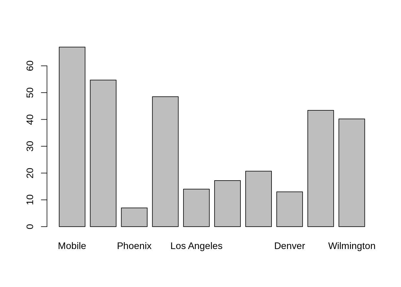
As you can see, the x-axis labels are bad. What if we turn the labels to be vertical?
barplot(precip[1:10], las=2)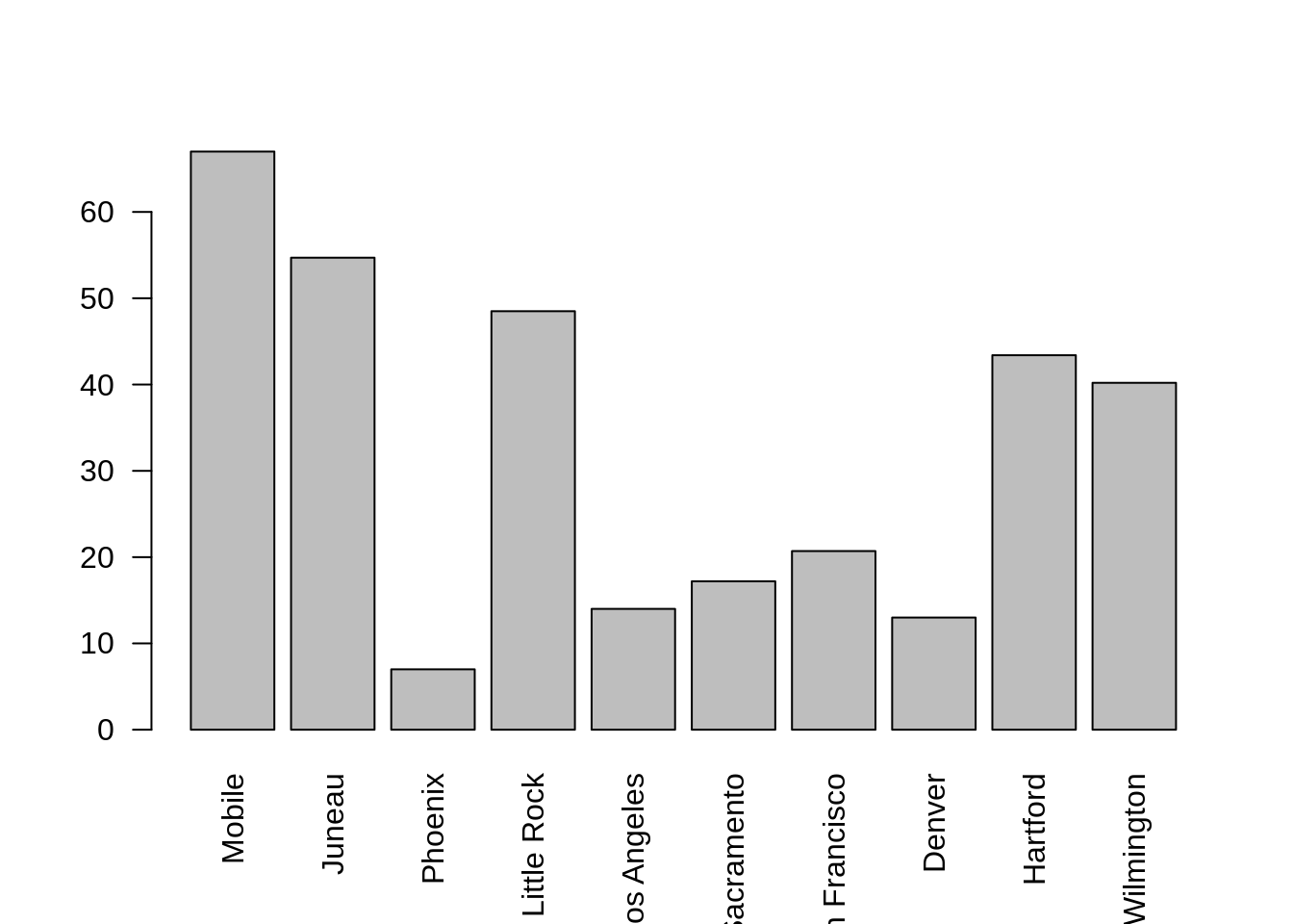
Much better, however, some of the longer names go off of the plot. Let's fix this:
par(oma=c(3,0,0,0)) # oma stands for outer margins. We increase the bottom margin to 3.
barplot(precip[1:10], las=2)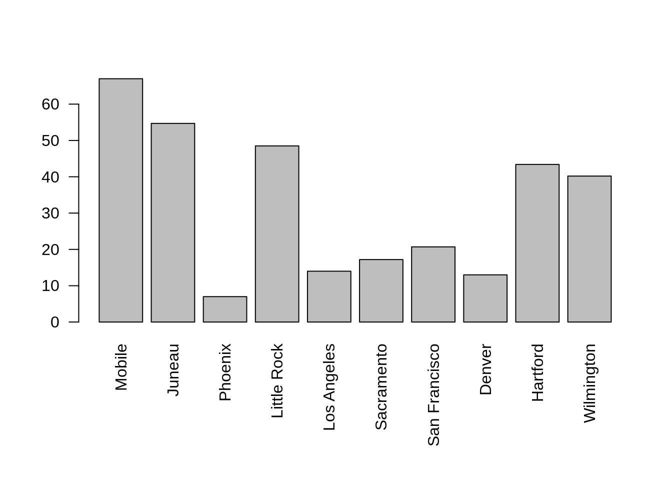
This is even better, however, it would be nice to have a title and axis label(s).
par(oma=c(3,0,0,0)) # oma stands for outer margins. We increase the bottom margin to 3.
barplot(precip[1:10], las=2, main="Average Precipitation", ylab="Inches of rain")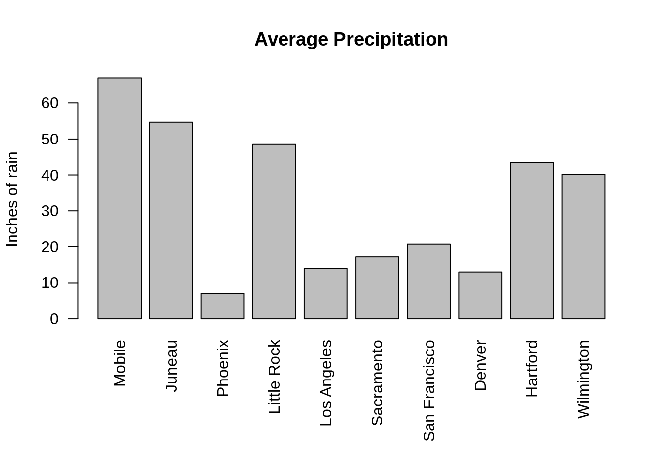
We are getting there. Let's add some color.
par(oma=c(3,0,0,0)) # oma stands for outer margins. We increase the bottom margin to 3.
barplot(precip[1:10], las=2, main="Average Precipitation", ylab="Inches of rain", col="blue")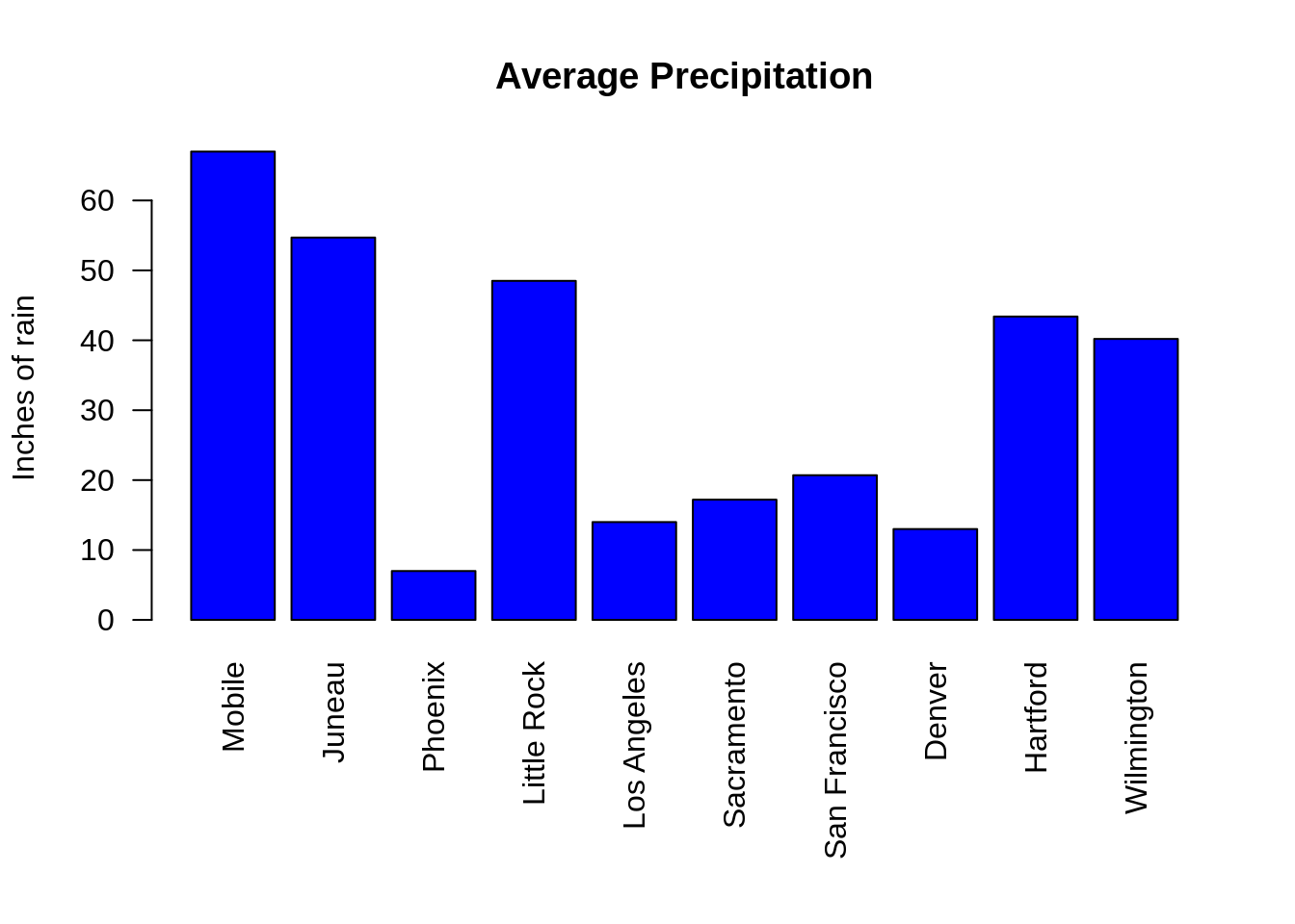
What if we want different colors for the different cities?
library(RColorBrewer)
par(oma=c(3,0,0,0)) # oma stands for outer margins. We increase the bottom margin to 3.
colors <- brewer.pal(10, "Set3")
barplot(precip[1:10], las=2, main="Average Precipitation", ylab="Inches of rain", col=colors)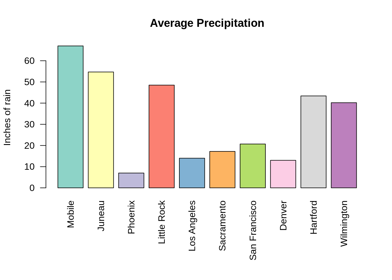
What if instead of x-axis labels, we want to use a legend?
library(RColorBrewer)
par(oma=c(0,0,0,0)) # oma stands for outer margins. We increase the bottom margin to 3.
colors <- brewer.pal(10, "Set3")
barplot(precip[1:10], las=2, main="Average Precipitation", ylab="Inches of rain", col=colors, legend=T, names.arg=F)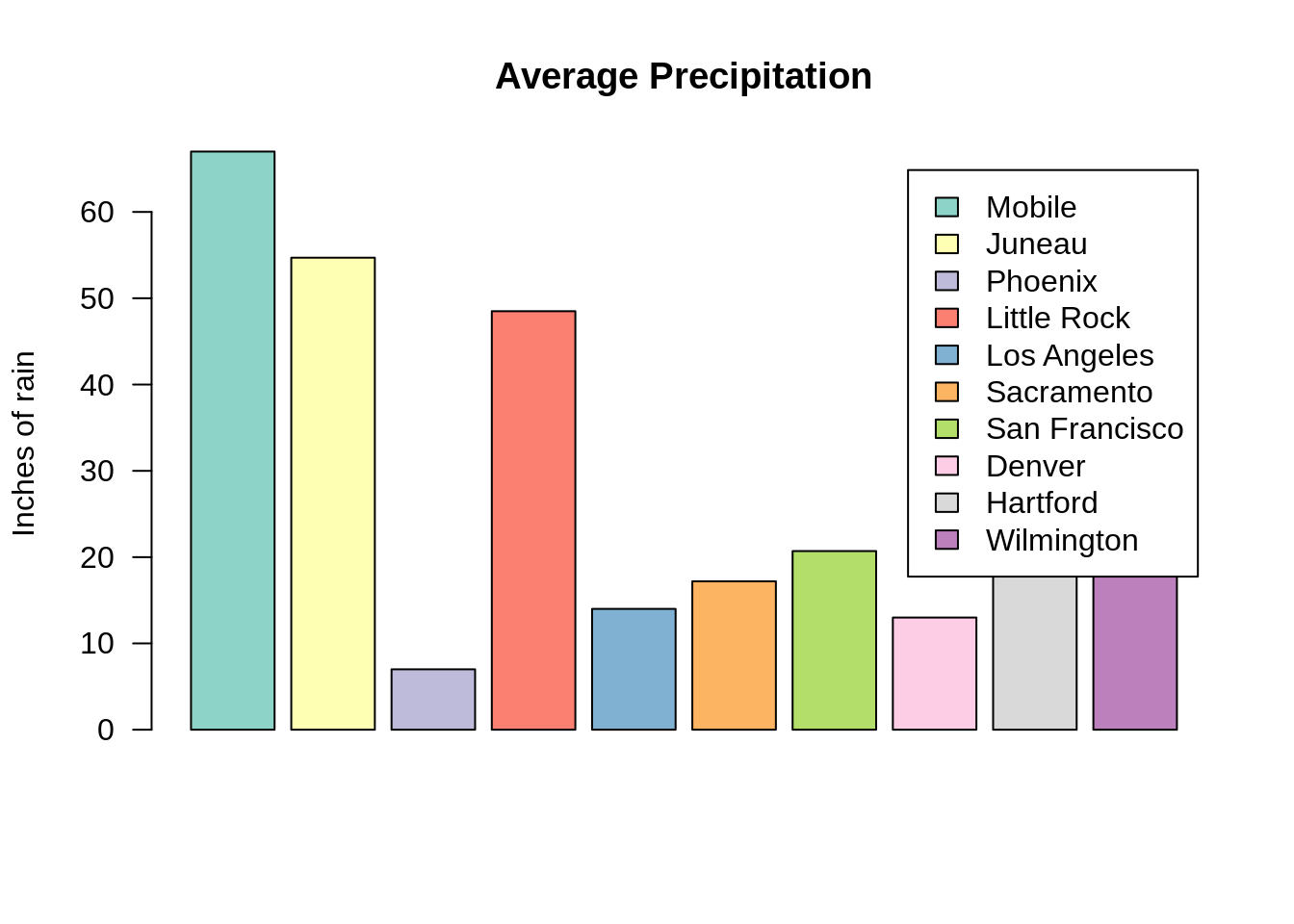
Pretty good, but now we don't need so much space at the bottom, and we need to make space for that legend. We use xlim to increase the x-axis, and args.legend to move the position of the legend along the x and y axes.
library(RColorBrewer)
colors <- brewer.pal(10, "Set3")
barplot(precip[1:10], las=2, main="Average Precipitation", ylab="Inches of rain", col=colors, legend=T, names.arg=F, xlim=c(0, 15), args.legend=list(x=16.5, y=46))
It's looking good, let's remove the box around the legend:
library(RColorBrewer)
colors <- brewer.pal(10, "Set3")
barplot(precip[1:10], las=2, main="Average Precipitation", ylab="Inches of rain", col=colors, legend=T, names.arg=F, xlim=c(0, 15), args.legend=list(x=16.5, y=46, bty="n"))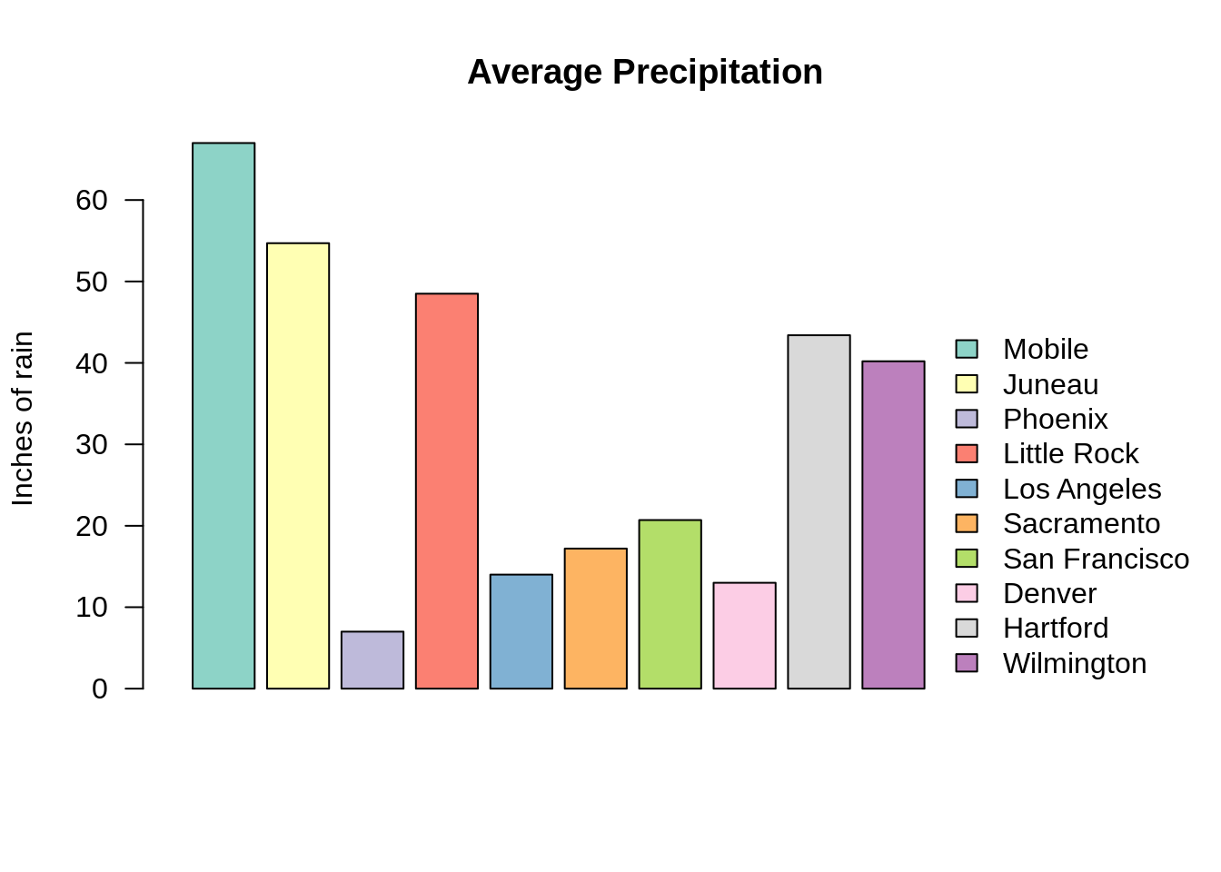
boxplot
boxplot is a function that creates a box and whisker plot, given some grouped data. The following is an example using the trees dataset.
First, we break our data into groups based on height.
dat <- trees
dat$size <- cut(trees$Height, breaks=c(0,76,100))
levels(dat$size) <- c("short", "tall")Next, we start with a box plot:
boxplot(dat$Girth ~ dat$size)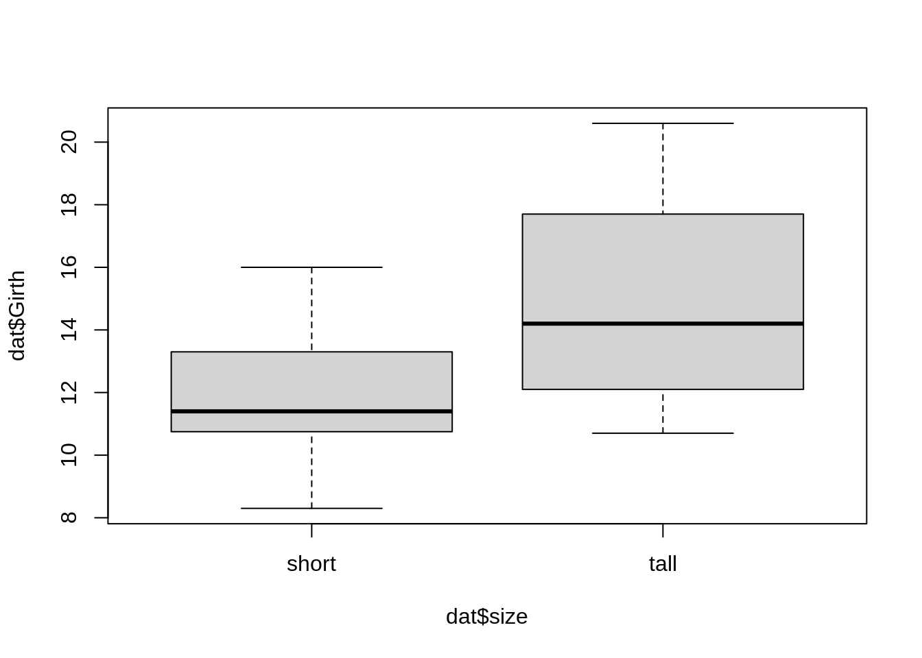
Let's spruce things up with proper labels:
boxplot(dat$Girth ~ dat$size, main="Tree girth", ylab="Girth in Inches", names=c("Short", "Tall"), xlab="")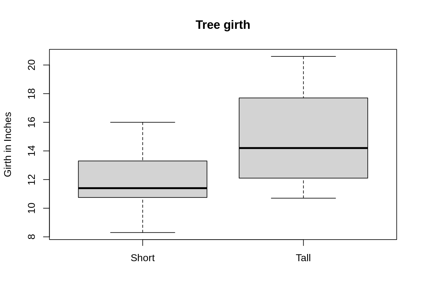
Let's add color:
boxplot(dat$Girth ~ dat$size, main="Tree girth", ylab="Girth in Inches", names=c("Short", "Tall"), xlab="", border="darkgreen", col="lightgreen")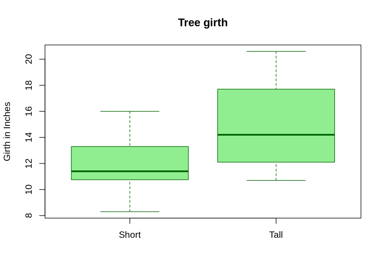
pie
pie is a function that creates a piechart.pie charts are used to display categorical data. The following is an example using the USPersonalExpenditure dataset.
First, let's get the mean expenditure:
# Quick look at data:
USPersonalExpenditure## 1940 1945 1950 1955 1960
## Food and Tobacco 22.200 44.500 59.60 73.2 86.80
## Household Operation 10.500 15.500 29.00 36.5 46.20
## Medical and Health 3.530 5.760 9.71 14.0 21.10
## Personal Care 1.040 1.980 2.45 3.4 5.40
## Private Education 0.341 0.974 1.80 2.6 3.64# Mean expenditure
expenditure <- rowMeans(USPersonalExpenditure)Now, we can create our pie chart.
pie(expenditure)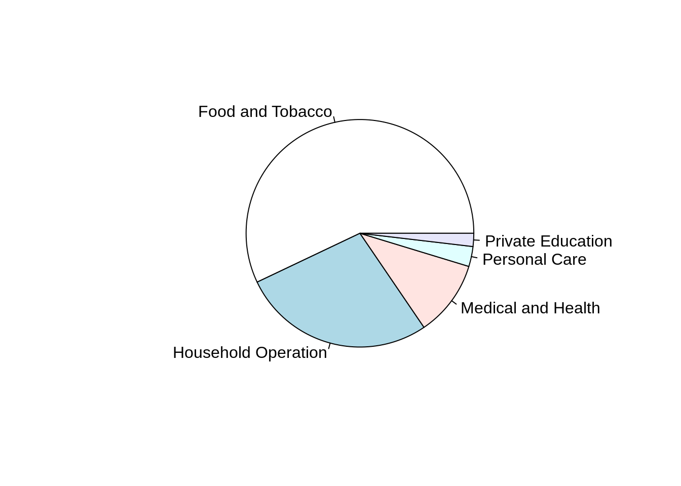
Let's use some different colors!
pie(expenditure, col = c("#8E6F3E", "#1c5253","#23395b","#6F727B", "#F97B64"))
Let's add the percentages next to the names. To do so, we must first get those values:
# calculating percentages
expenditure_percentage <- 100*expenditure/sum(expenditure)
# rounding percentages to 2 decimal places
expenditure_percentage <- round(expenditure_percentage, 2)
# combining names with percentages
expenditure_names <- paste0(names(expenditure), " (", expenditure_percentage, "%)")
# creating new labels
pie(expenditure, labels = expenditure_names, col = c("#8E6F3E", "#1c5253","#23395b","#6F727B", "#F97B64"))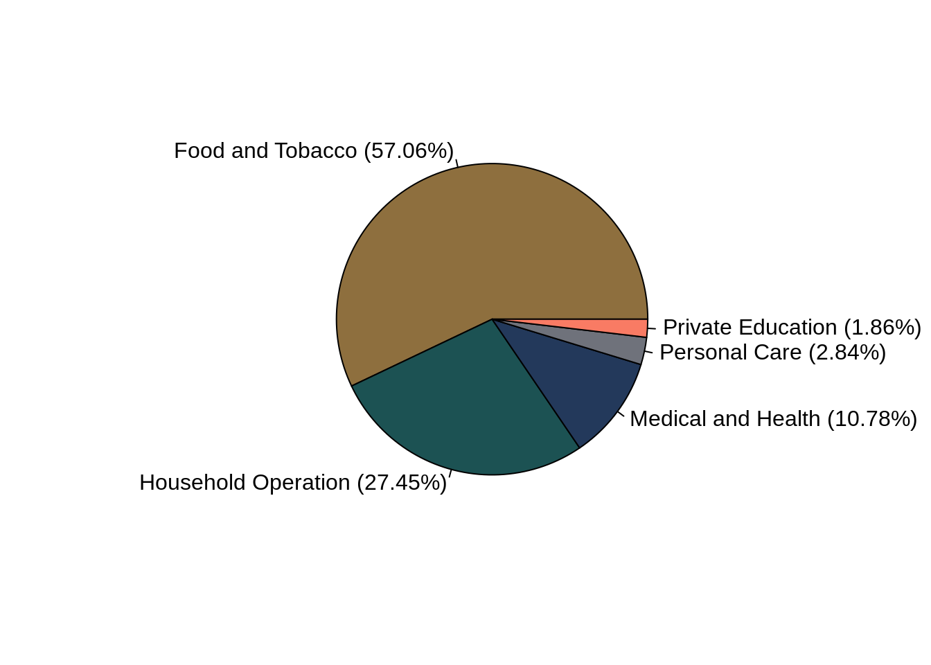
Let's add a title:
pie(expenditure, labels = expenditure_names, col = c("#8E6F3E", "#1c5253","#23395b","#6F727B", "#F97B64"), main = "Mean US expenditure from 1940 to 1960")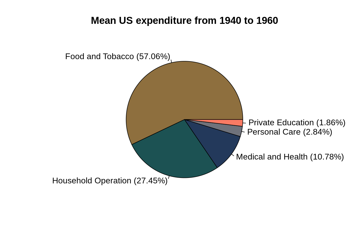
dotchart
dotchart draws a Cleveland dot plot.
Fun Fact: Dr. Cleveland is a Distinguished Professor in the Statistics department at Purdue University!
The following is an example using the built-in HairEyeColor dataset.
First, let's consider only individuals with black hair.
# Selecting only individuals with black hair
black_hair = HairEyeColor[1,,]
# Summing both Male and Female.
black_hair = rowSums(black_hair)Now we can create our dotchart.
dotchart(black_hair)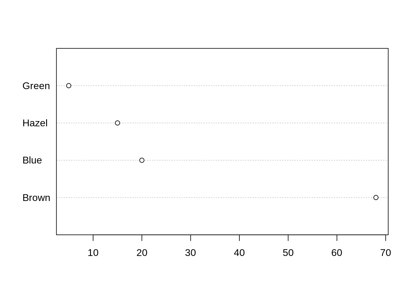
Let's add a title, and labels to the x-axis and the y-axis.
dotchart(black_hair, main='Eye color for individuals with black hair', xlab='Count', ylab='Eye color')
That's better. Let's arrange the data in an ascending manner.
# re-ordering the data
black_hair <- sort(black_hair)
dotchart(black_hair, main='Eye color for individuals with black hair', xlab='Count', ylab='Eye color') 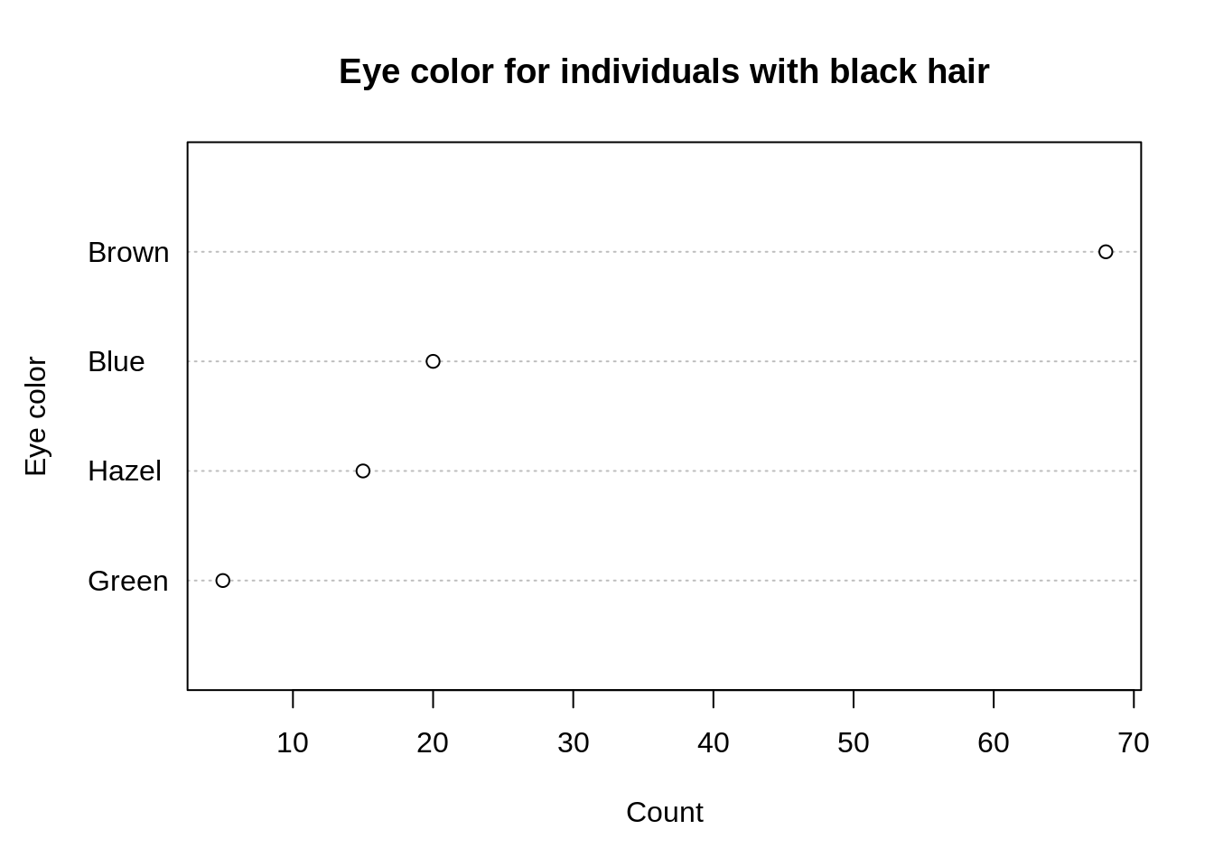
How about some color?
dotchart(black_hair, main='Eye color for individuals with black hair', xlab='Count', ylab='Eye color', bg='orange')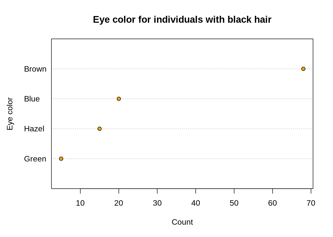
plot
plot is a generic plotting function. It creates scatter plots as well as line plots. The argument type allows you to define the type of plot that should be drawn. Most common types are "p" for points (default), "l" for lines, and "b" for both.
Scatter plots
Below is an example using the built-in Orange dataset.
plot(Orange$age, Orange$circumference)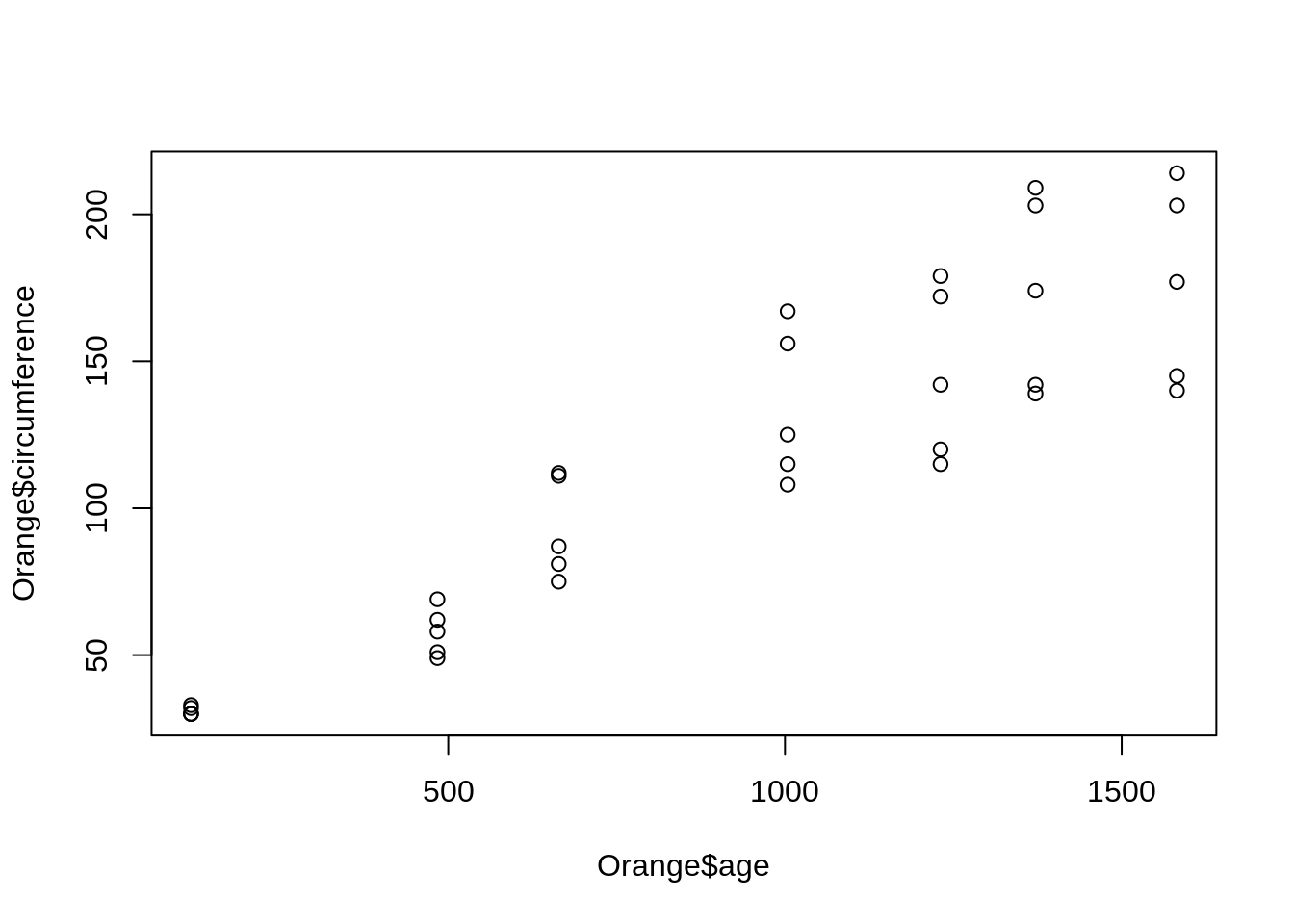
The labels for x-axis and y-axis can be improved!
plot(Orange$age, Orange$circumference, xlab='Tree age', ylab='Tree circumference')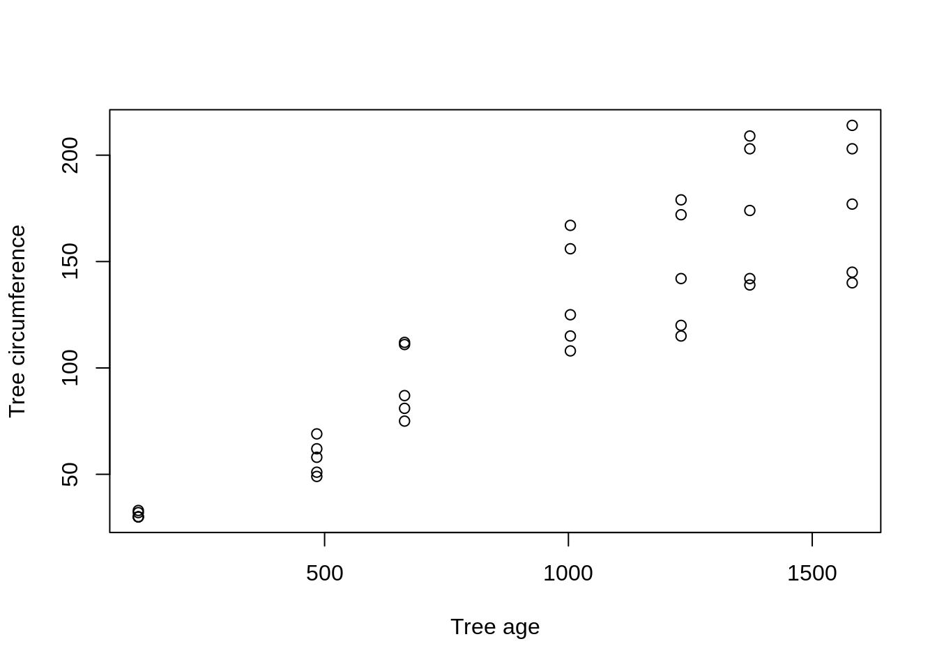
We can also add a title.
plot(Orange$age, Orange$circumference, xlab='Tree age', ylab='Tree circumference', main='Growth of orange trees')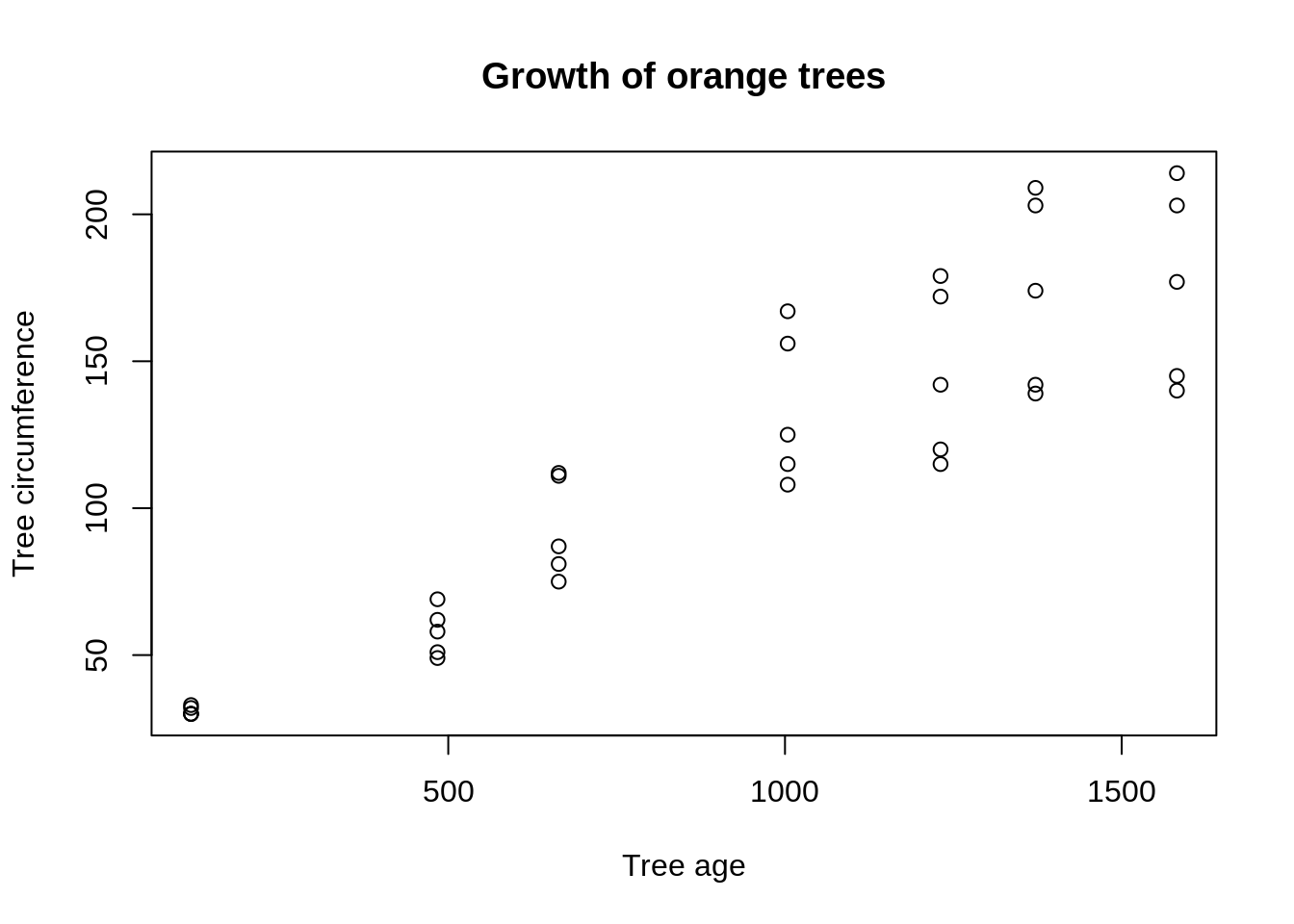
The argument pch specifies what symbol to use when plotting. pch set at "21" enables us to have colored circles. We can specify both the border and fill colors. Let's give it a try.
plot(Orange$age, Orange$circumference, xlab='Tree age', ylab='Tree circumference', main='Growth of orange trees', pch=21, bg='lightblue', col='tomato')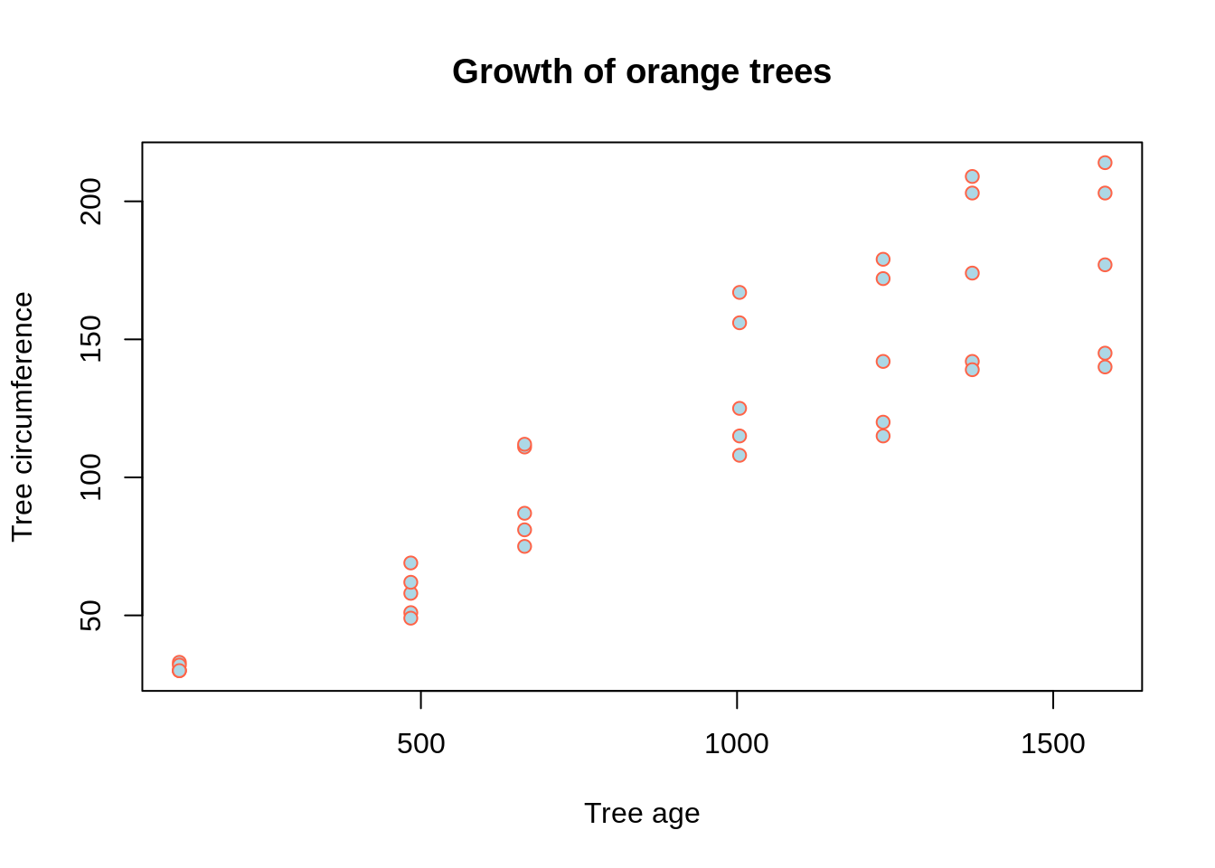
How about coloring the points based on the tree?
plot(Orange$age, Orange$circumference, xlab='Tree age', ylab='Tree circumference', main='Growth of orange trees', pch=21, bg=Orange$Tree)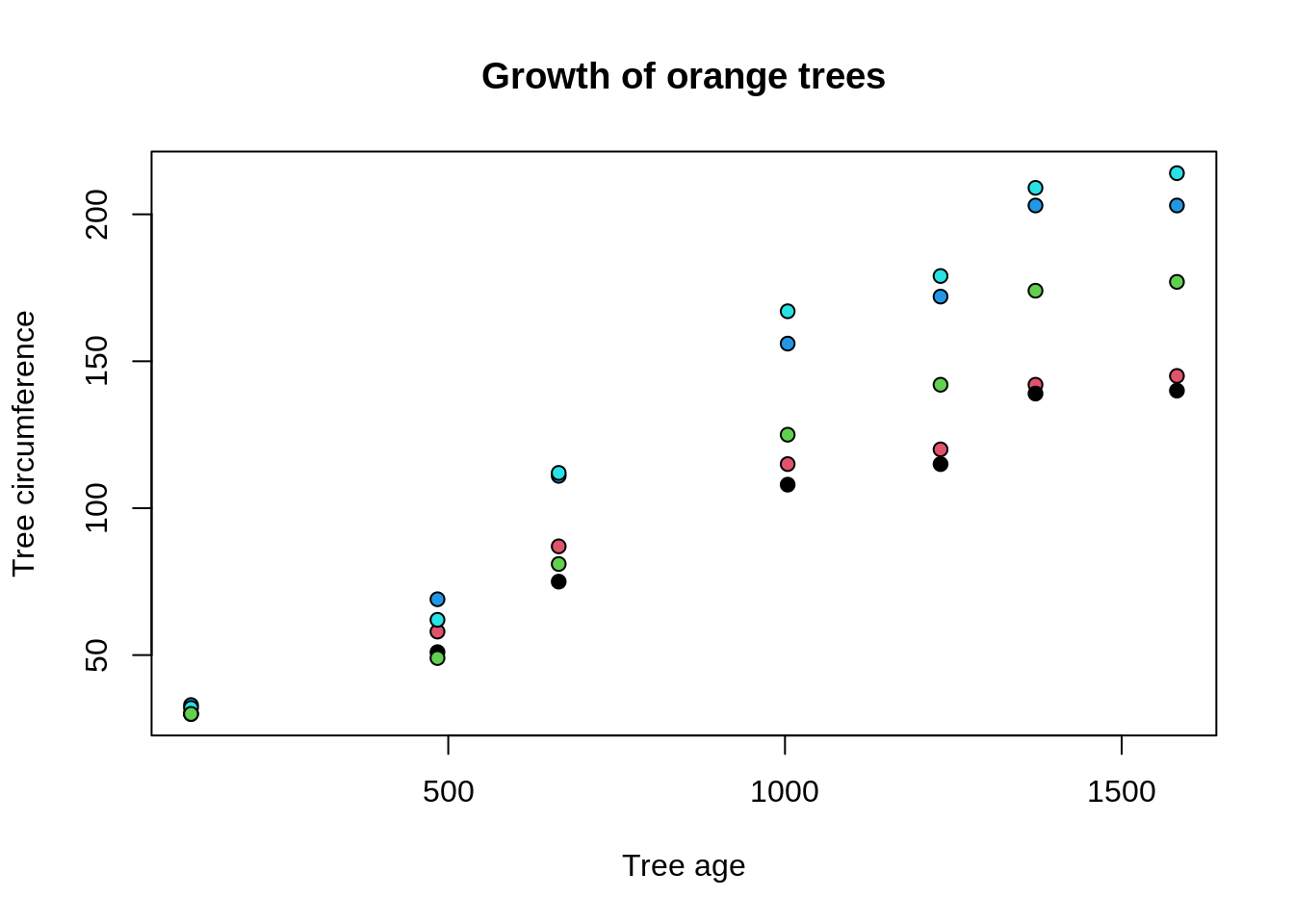
geom_point
To make an equivalent graphic using ggplot:
ggplot(Orange, aes(x=age, y=circumference)) +
geom_point()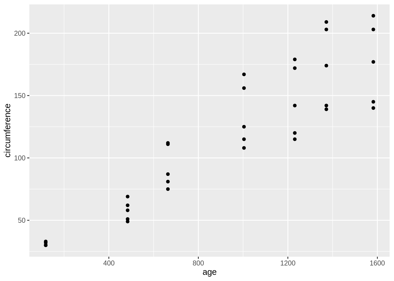
Here, the first argument to ggplot is our dataset, Orange. The second argument, aes(x=age, y=circumference) are our aesthetic mappings. The aesthetic mappings specifies how we map certain variables/columns from our Orange dataset to grapic components. In this case, we say the x-axis has the age column and the y-axis has the circumference column. Then, we add geom_point, which is a layer with dots to represent the data!
Like before, our labels can be improved.
ggplot(Orange, aes(x=age, y=circumference)) +
geom_point() +
labs(x="Tree age", y="Tree circumference")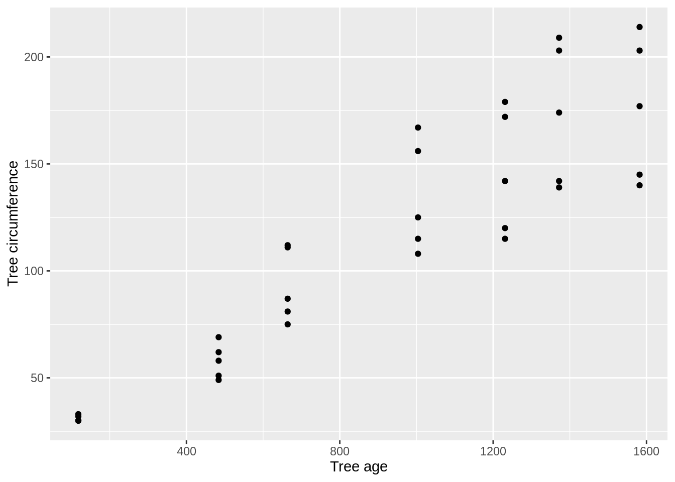
Here, we added labels using labs. We could also add a title, or even subtitle, using labs.
ggplot(Orange, aes(x=age, y=circumference)) +
geom_point() +
labs(x="Tree age", y="Tree circumference", title="Growth of orange trees", subtitle="An exciting plot")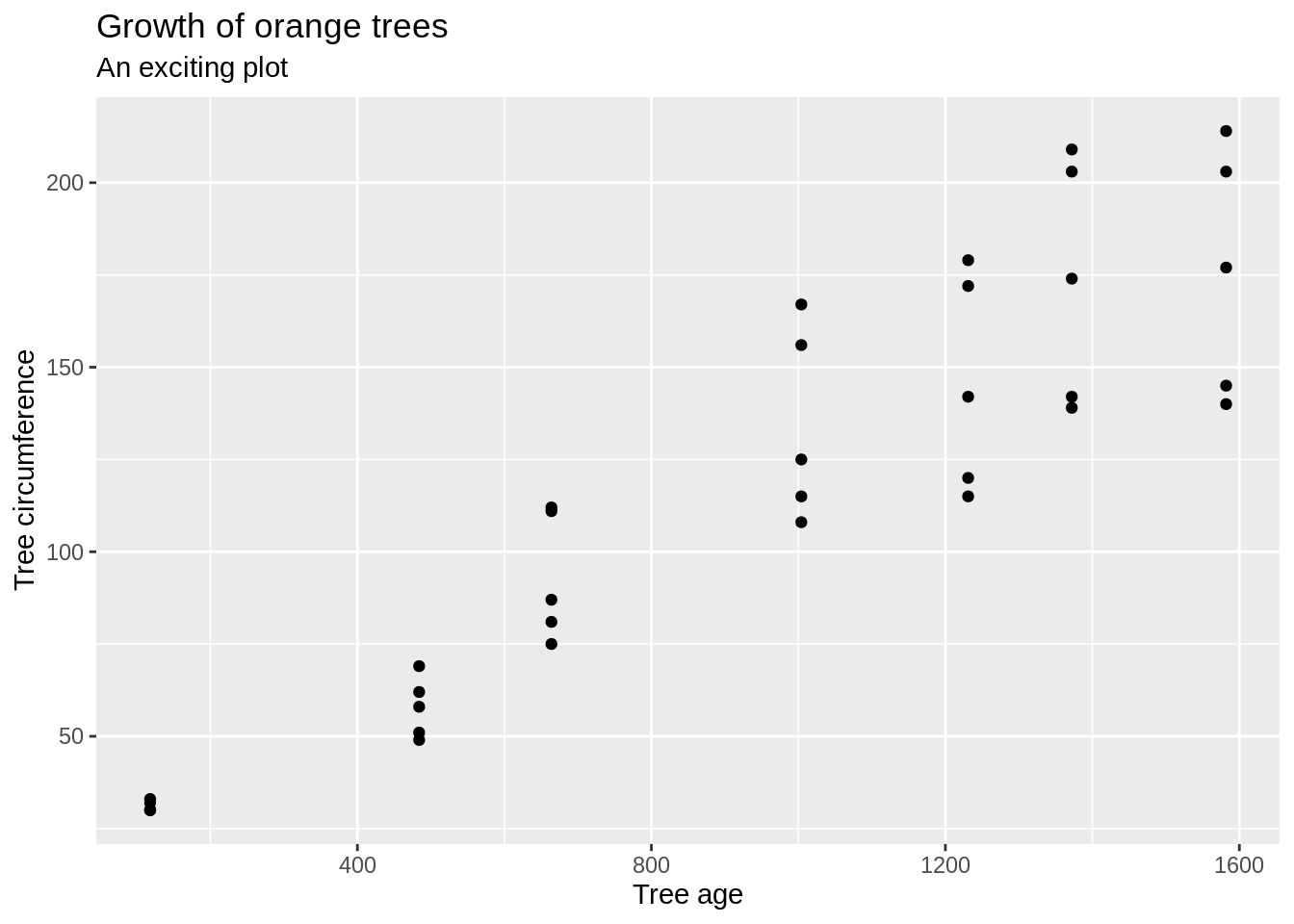
If we wanted to change the color of the dots, we could do so using the color option in the aesthetics:
ggplot(Orange, aes(x=age, y=circumference, color="tomato")) +
geom_point() +
labs(x="Tree age", y="Tree circumference", title="Growth of orange trees", subtitle="An exciting plot")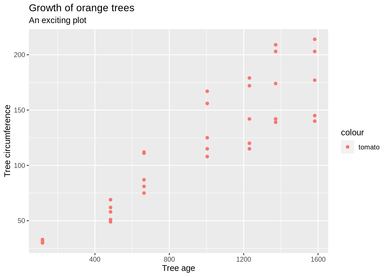
As you can see, this creates a legend by default. To remove the legend, we can specify an option to geom_point to not show a legend.
ggplot(Orange, aes(x=age, y=circumference, color="tomato")) +
geom_point(show.legend=F) +
labs(x="Tree age", y="Tree circumference", title="Growth of orange trees", subtitle="An exciting plot")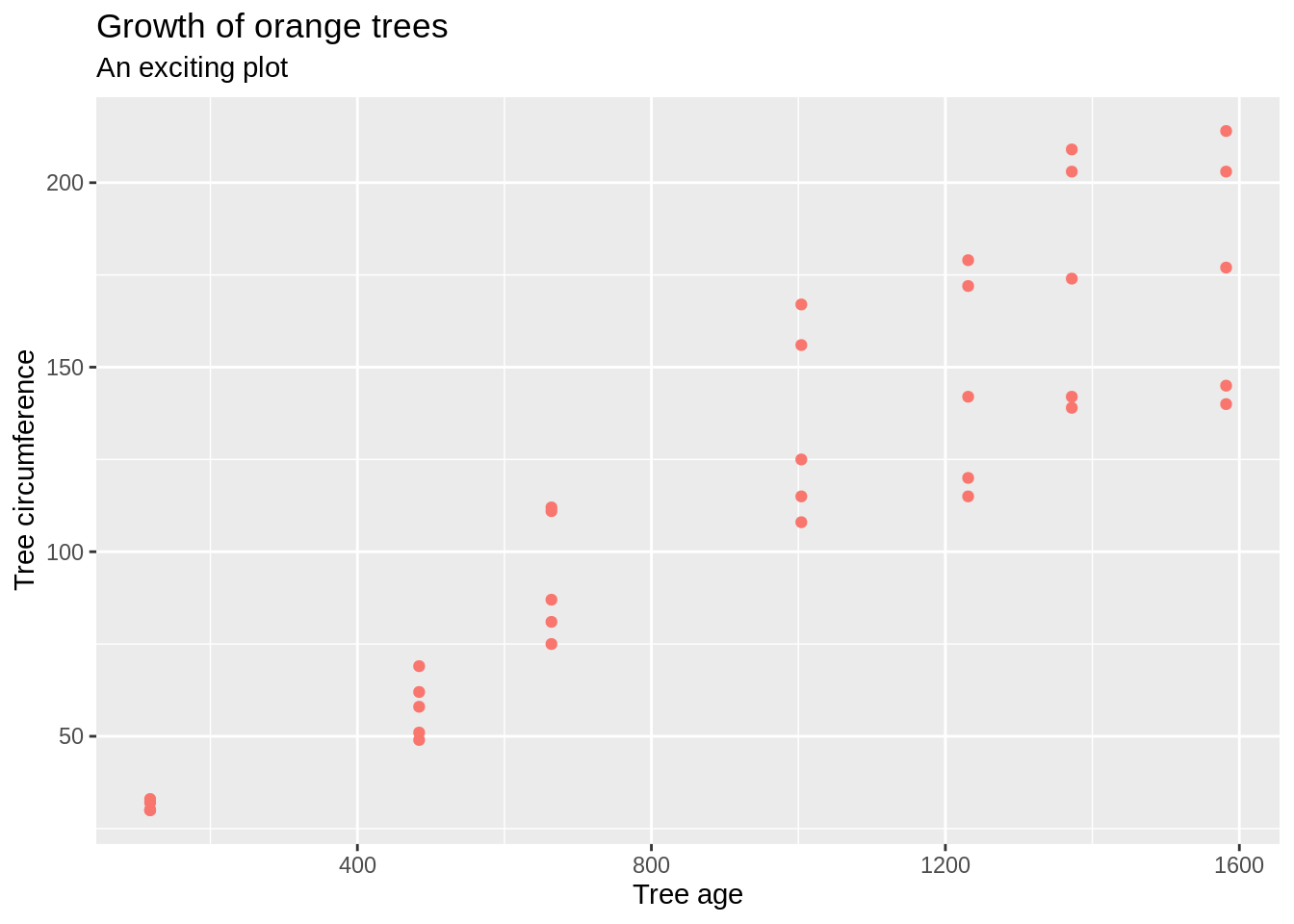
What if we wanted to color the points based on the tree (in the Tree column)?
ggplot(Orange, aes(x=age, y=circumference, color=Tree)) +
geom_point() +
labs(x="Tree age", y="Tree circumference", title="Growth of orange trees", subtitle="An exciting plot")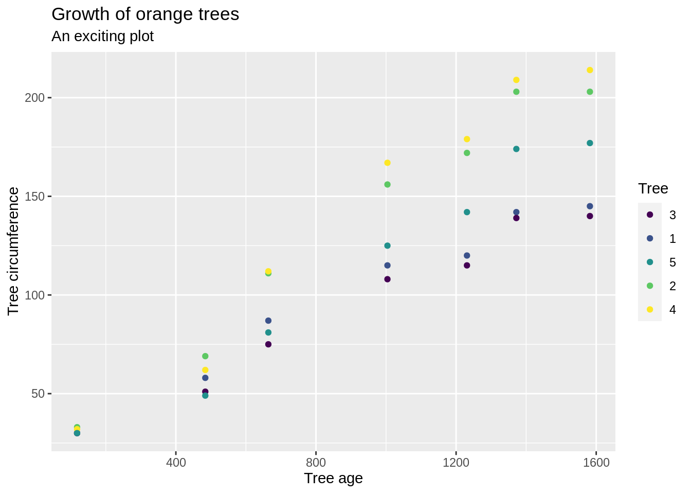
Here, the legend is more important, so we remove the show.legend=F option to geom_point. Unfortunately, our legend is out of order. The order of the legend is based on the levels of the column. For example, here the levels are in the order: 3,1,5,2,4:
levels(Orange$Tree)## [1] "3" "1" "5" "2" "4"To modify the order of the legend, simply change the order of the levels:
new_orange <- Orange
new_orange$Tree <- factor(new_orange$Tree, levels = c(1,2,3,4,5))
ggplot(new_orange, aes(x=age, y=circumference, color=Tree)) +
geom_point() +
labs(x="Tree age", y="Tree circumference", title="Growth of orange trees", subtitle="An exciting plot")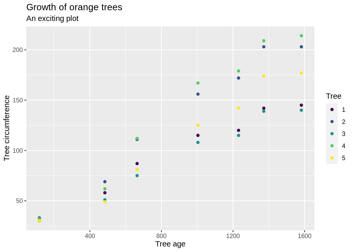
Line plots
Below is an example using the built-in Orange dataset.
plot(Orange$age, Orange$circumference, type='l')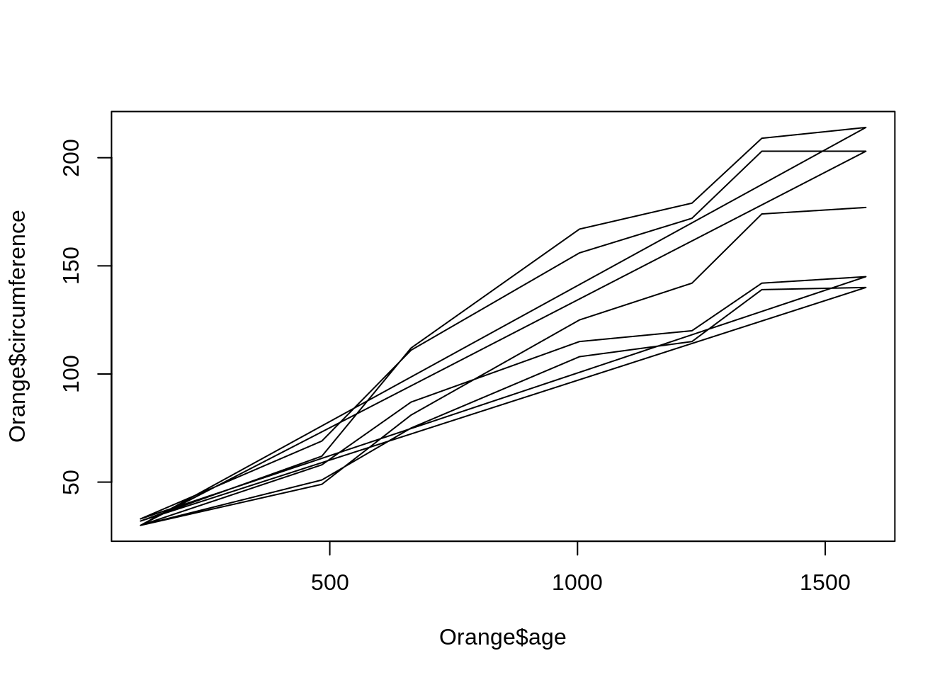
Let's fix the title and axes labels.
plot(Orange$age, Orange$circumference, type='l', xlab='Tree age', ylab='Tree circumference', main='Growth of orange trees')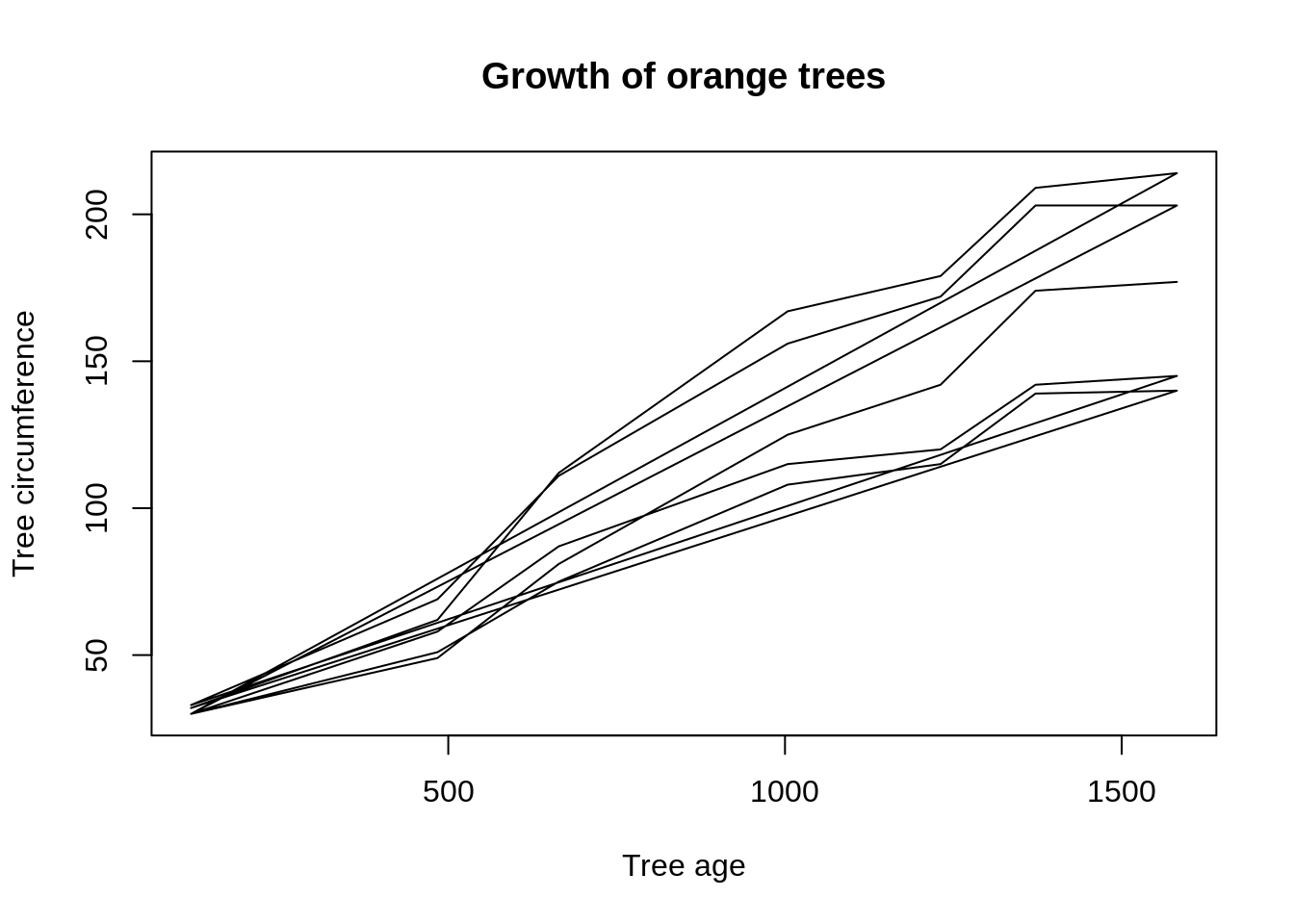
lty is an argument that allows us to change the linetype. This is the equivalent version of pch for lines. There 7 options: "blank", "solid", "dashed", "dotted", "dotdash", "longdash", and "twodash".
plot(Orange$age, Orange$circumference, type='l', xlab='Tree age', ylab='Tree circumference', main='Growth of orange trees', lty='longdash')
We can also modify the thickness of the lines using the argument lwd. Below is an example.
plot(Orange$age, Orange$circumference, type='l', xlab='Tree age', ylab='Tree circumference', main='Growth of orange trees', lty='longdash', lwd=1.5)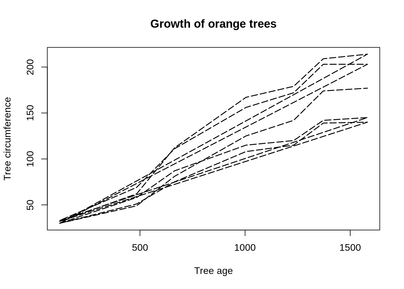
lines
lines draws additional lines to an existing graphic. For example, let's add lines to our orange scatter plot.
# Original chart
plot(Orange$age, Orange$circumference, xlab='Tree age', ylab='Tree circumference', main='Growth of orange trees', pch=21, bg=Orange$Tree)
# Adding lines
lines(Orange$age, Orange$circumference)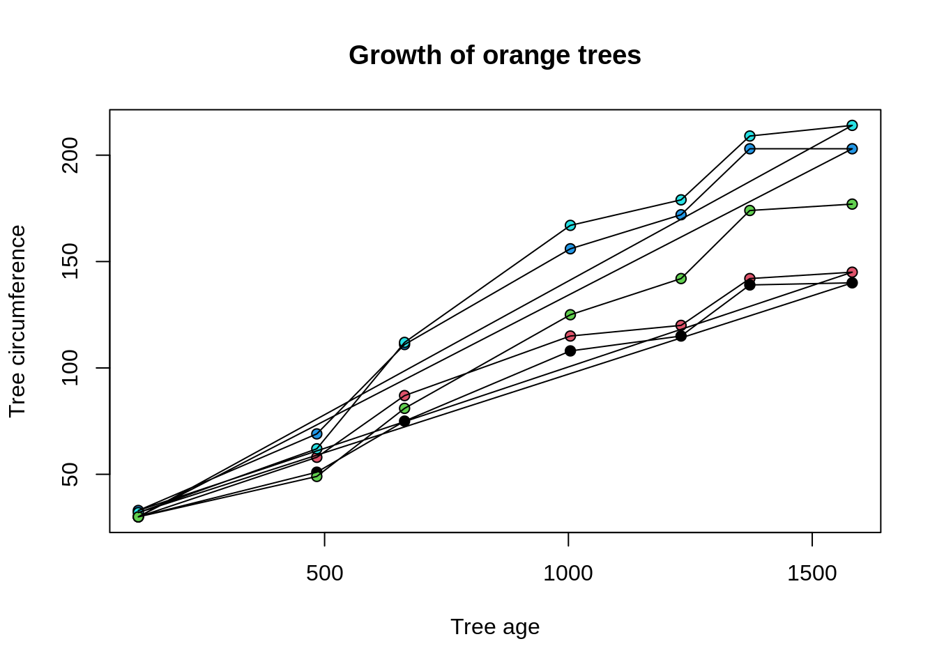
The lines are too strong. It will probably be nicer to have them in a different type, such as "dotted".
# Original chart
plot(Orange$age, Orange$circumference, xlab='Tree age', ylab='Tree circumference', main='Growth of orange trees', pch=21, bg=Orange$Tree)
# Adding lines
lines(Orange$age, Orange$circumference, lty='dotted')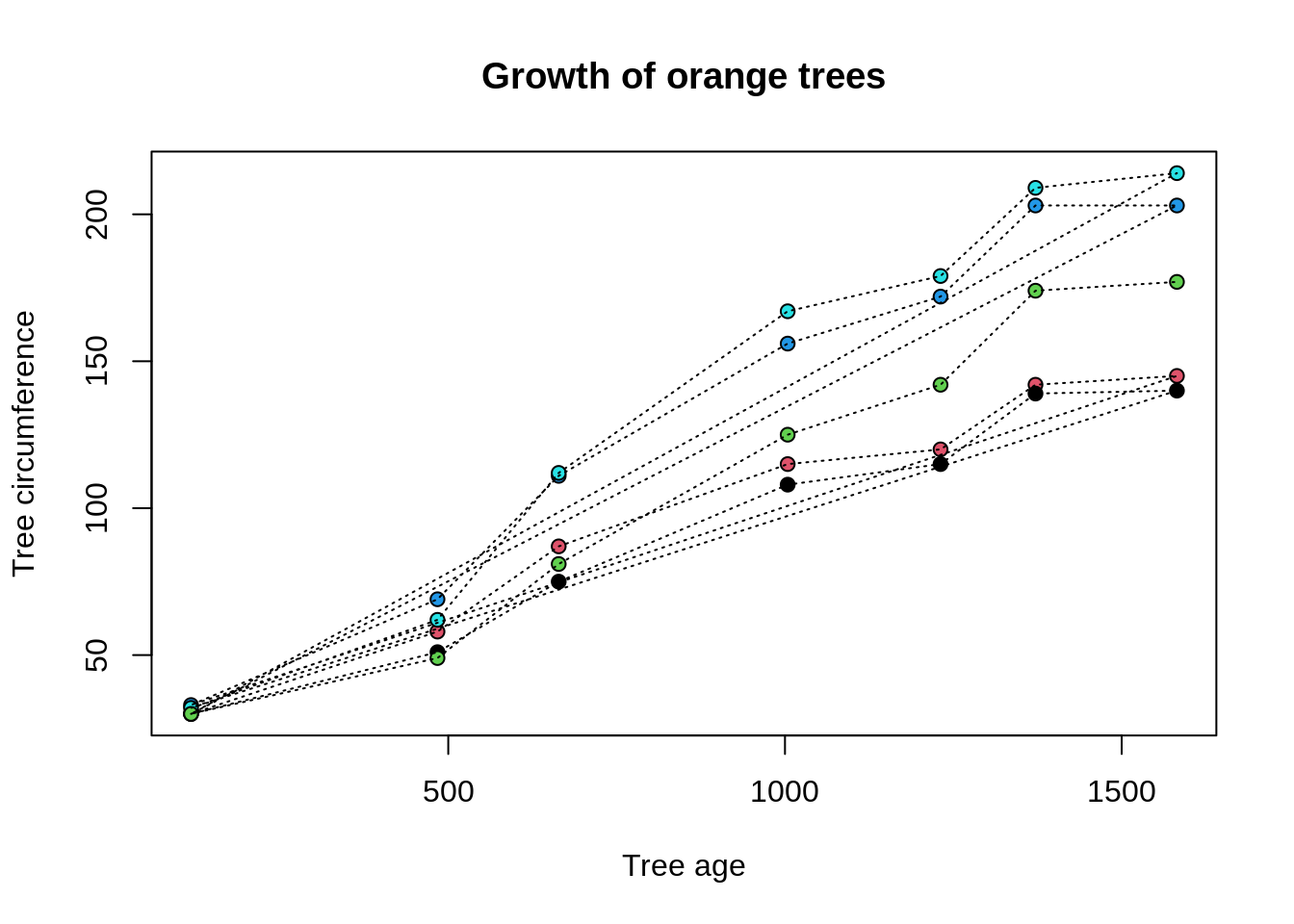
Note that we could continue to add lines. For example, suppose we now want to add the average orange growth line.
# Original chart
plot(Orange$age, Orange$circumference, xlab='Tree age', ylab='Tree circumference', main='Growth of orange trees', pch=21, bg=Orange$Tree)
# Adding lines
lines(Orange$age, Orange$circumference, lty='dotted')
# Getting average growth
avg_growth <- tapply(Orange$circumference, Orange$age, mean)
# Adding the average growth line
lines(unique(Orange$age), avg_growth, col='tomato', lwd=2.5)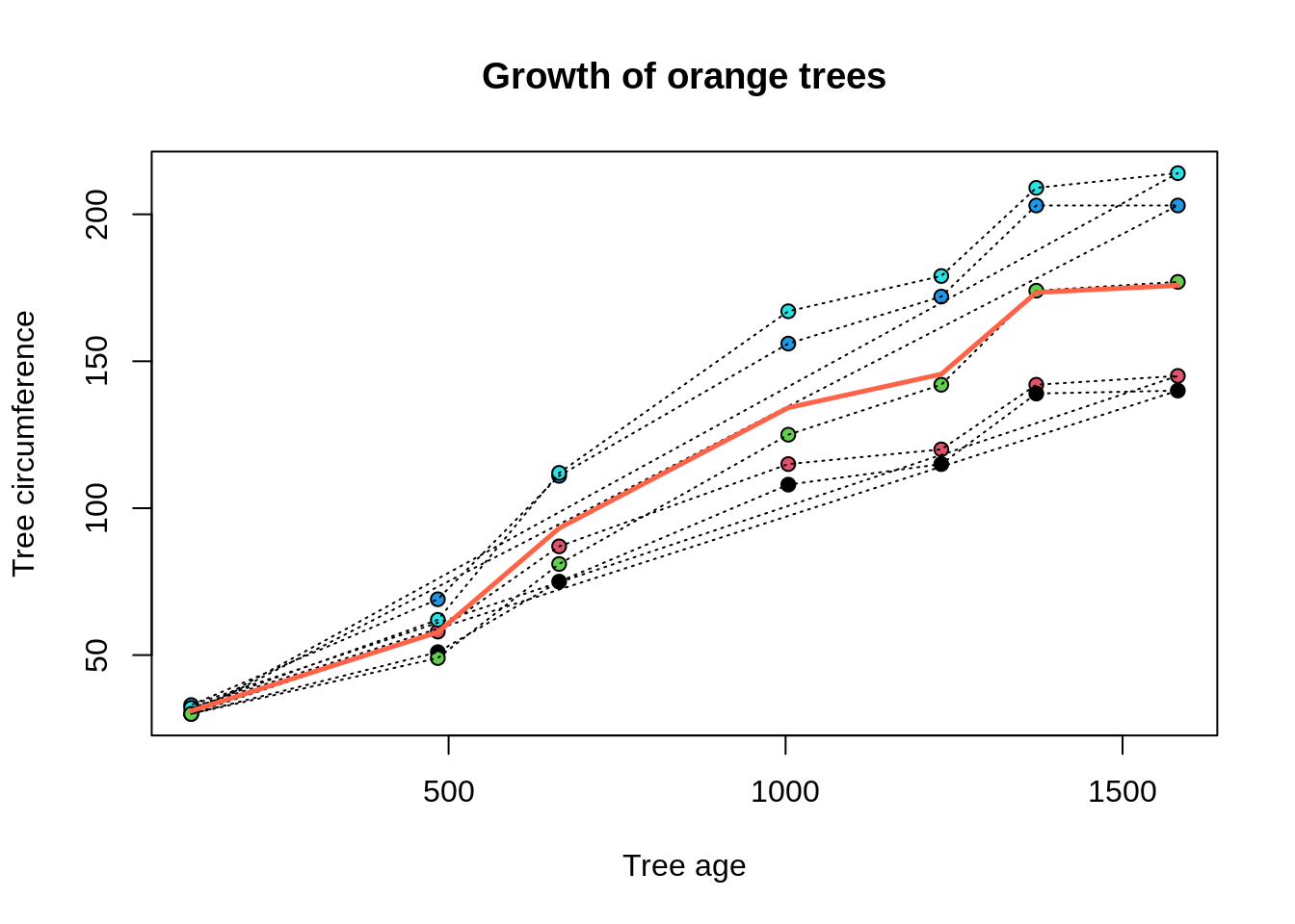
We can add lines to any plot. Here is an example adding lines to a barplot.
# Original chart
par(oma=c(3,0,0,0))
barplot(precip[1:10], las=2)
# Adding a dot-dash vertical line
lines(0:12, rep(20,13), lty='longdash') 
points
points draws points on an existing graphic. For example, let's add the points to the line plot we did earlier.
# Original chart
plot(Orange$age, Orange$circumference, type='l', xlab='Tree age', ylab='Tree circumference', main='Growth of orange trees')
# Adding points
points(Orange$age, Orange$circumference)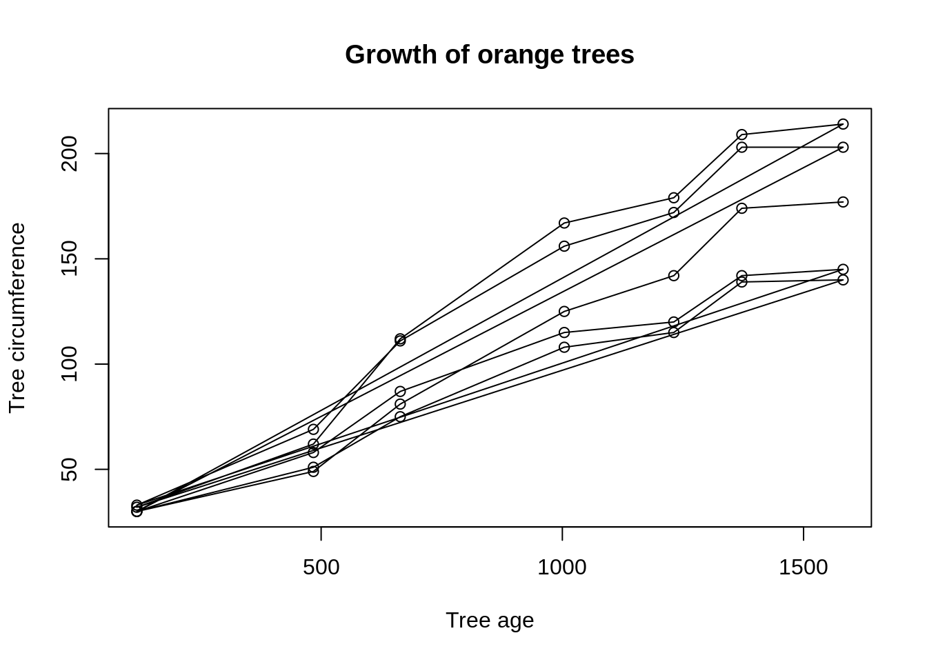
It's hard to see the points. It would help to have the lines be dark grey, and have the points be colored.
# Original chart with grey lines
plot(Orange$age, Orange$circumference, type='l', xlab='Tree age', ylab='Tree circumference', main='Growth of orange trees', col='grey')
# Adding points
points(Orange$age, Orange$circumference, pch=20, col='tomato')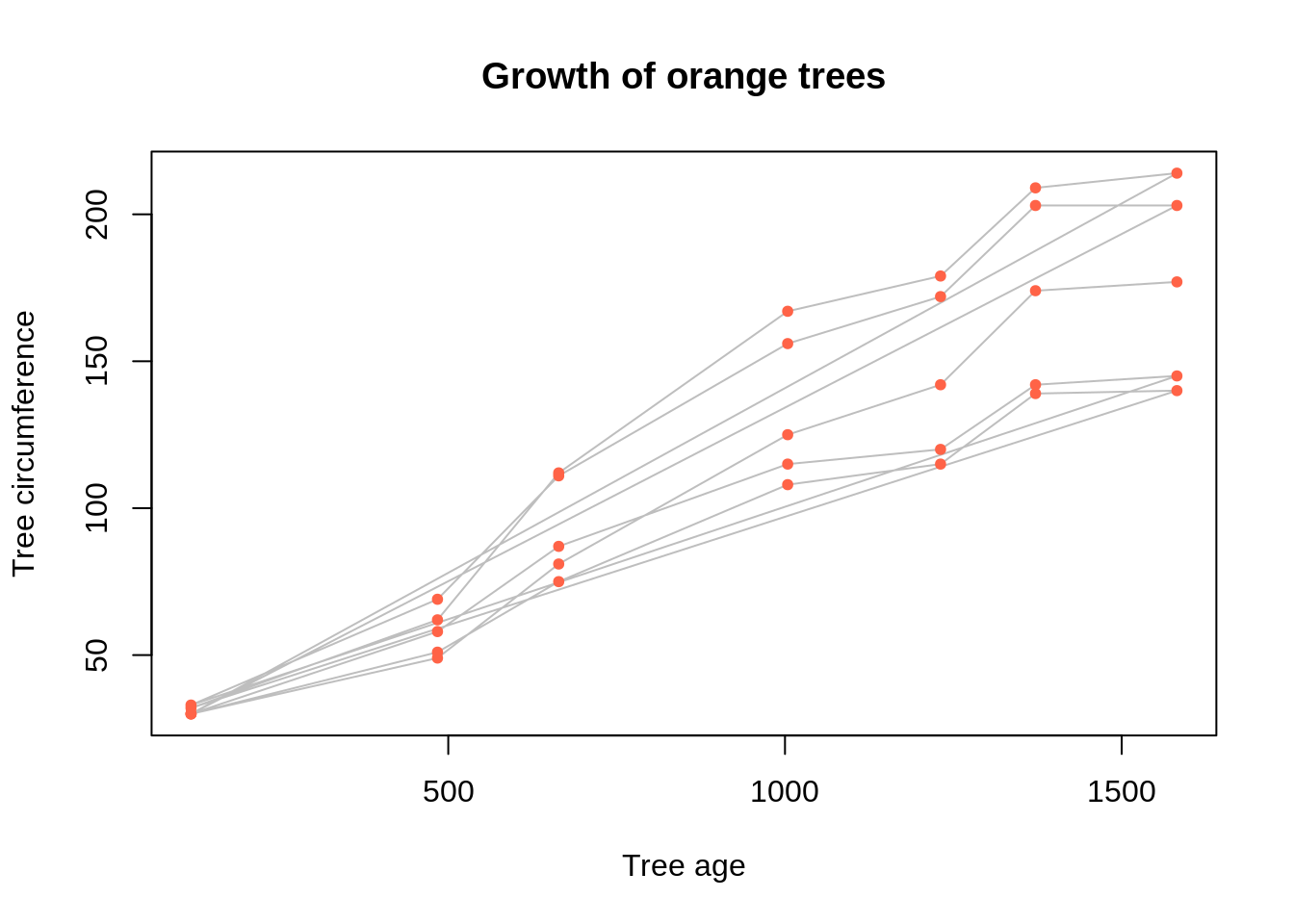
Much better!
Similar to lines, we can add points to any plot. Here is an example adding lines to a barplot.
# Original chart
par(oma=c(3,0,0,0))
barplot(precip[1:10], las=2)
# Adding a dot-dash vertical line
x_values <- seq(1,10, length=10) + seq(-.3,1.5,length=10) # adjusting x positions
points(x_values, precip[1:10], pch=21, bg='steelblue') 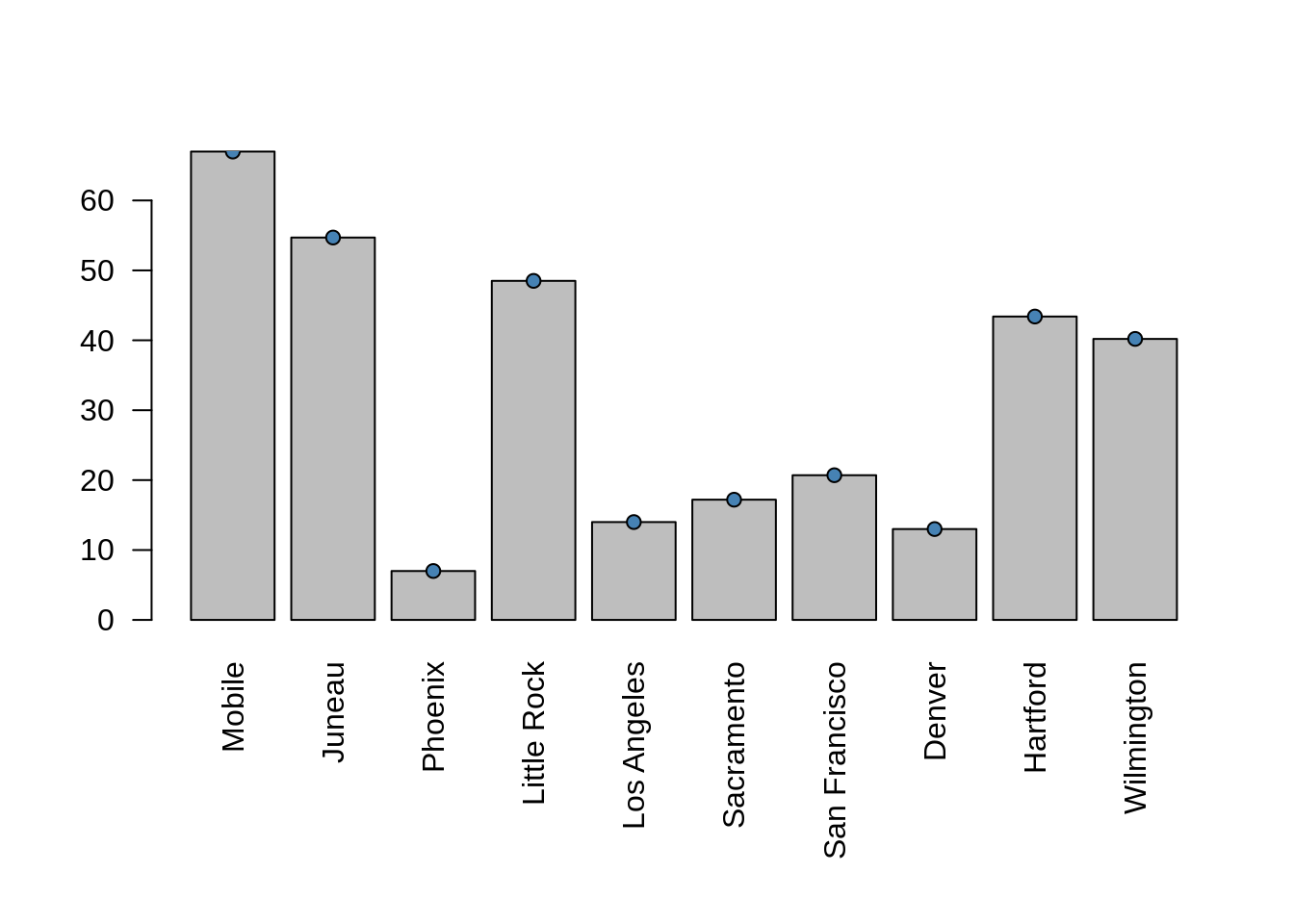
abline
abline is similar to the lines function. Below are some examples.
Let's add a Y=X line (with intercept=0 and slope=1).
# Original chart
plot(cars$speed, cars$dist, xlab="Speed (mph)", ylab="Stopping distance (ft)")
# Adding Y=X line
abline(a=0, b=1) # a = intercept, b=slope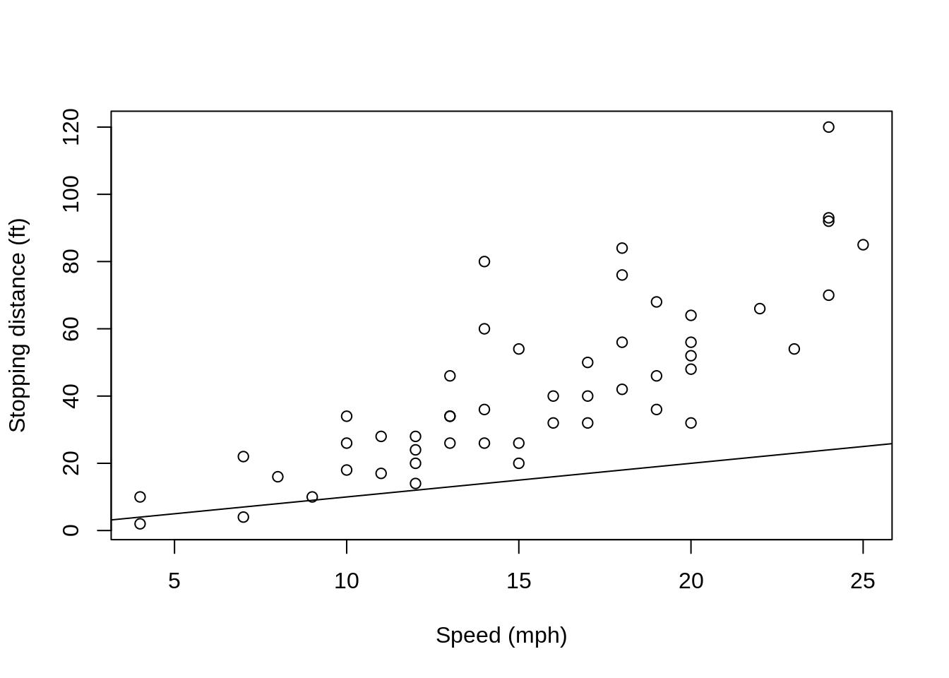
Let's add a horizontal line at 60.
# Original chart
plot(cars$speed, cars$dist, xlab="Speed (mph)", ylab="Stopping distance (ft)")
# Adding a dotted horizontal line
abline(h=60, lty='dotted') 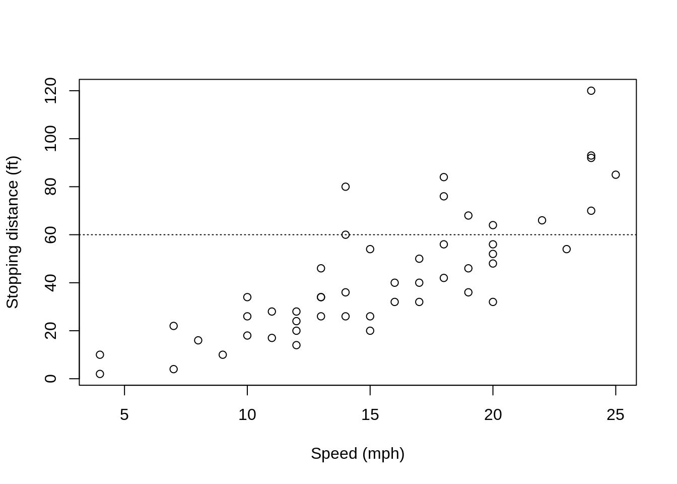
Let's add a vertical line at 15.
# Original chart
plot(cars$speed, cars$dist, xlab="Speed (mph)", ylab="Stopping distance (ft)")
# Adding a dot-dash vertical line
abline(v=15, lty='dotdash') 
As with lines and points, we can continue to add ablines.
# Original chart
plot(cars$speed, cars$dist, xlab="Speed (mph)", ylab="Stopping distance (ft)")
# Adding Y=X line
abline(a=0, b=1) # a = intercept, b=slope
# Adding a dotted horizontal line
abline(h=60, lty='dotted')
# Adding a dot-dash vertical line
abline(v=15, lty='dotdash') 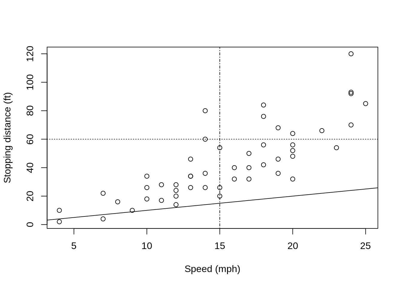
As lines and points we can add ablines to any plot. Here is an example adding lines to a dotchart.
# Original chart
dotchart(black_hair, main='Eye color for individuals with black hair', xlab='Count', ylab='Eye color', bg='orange')
# Adding a dot-dash vertical line
abline(v=15, lty='dotdash') 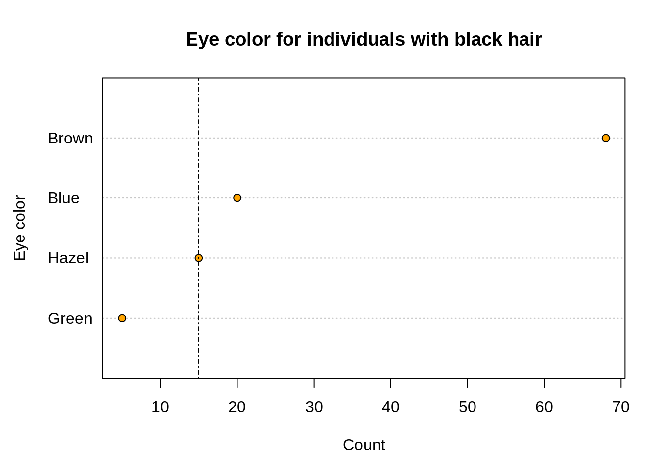
text
text enables us to add texts to our plots. Similarly to points,lines, and abline we can add text to any plot. For the example below, we will focus on scatter plots and the built-in dataset mtcars.
# Original chart
plot(mtcars$mpg, mtcars$disp, xlab='Miles/(US) gallon', ylab='Displacement (cu.in.)', pch=21, bg='orange')
# Text with some additional comments
# x and y enables us to select a location
text(x=29,y=460,'Note a downward trend')
How about making it italicized? We can change the font using the font argument. It takes 4 values: 1 or plain, 2 or bold, 3 or italic, 4 and bold-italic.
# Original chart
plot(mtcars$mpg, mtcars$disp, xlab='Miles/(US) gallon', ylab='Displacement (cu.in.)', pch=21, bg='orange')
# Text with some additional comments
text(x=29,y=460,'Note a downward trend', font=3)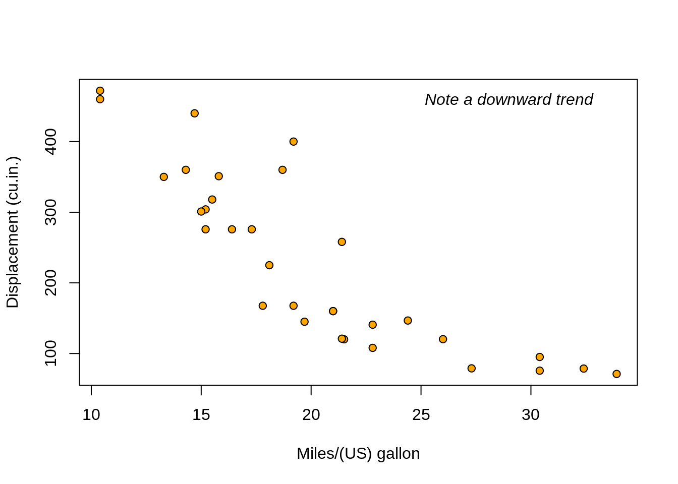
How about we add labels that show what cars are some (or all) of these points? We can do this using the argument labels.
# Original chart
plot(mtcars$mpg, mtcars$disp, xlab='Miles/(US) gallon', ylab='Displacement (cu.in.)', pch=21, bg='orange')
# Text with some additional comments
text(x=29,y=460,'Note a downward trend', font=3)
# Selecting some cars
subset_mtcars <- subset(mtcars, ((mpg>18&mpg<20)&disp>300))
# Label to some cars
text(x=subset_mtcars$mpg,y=subset_mtcars$disp,labels=row.names(subset_mtcars))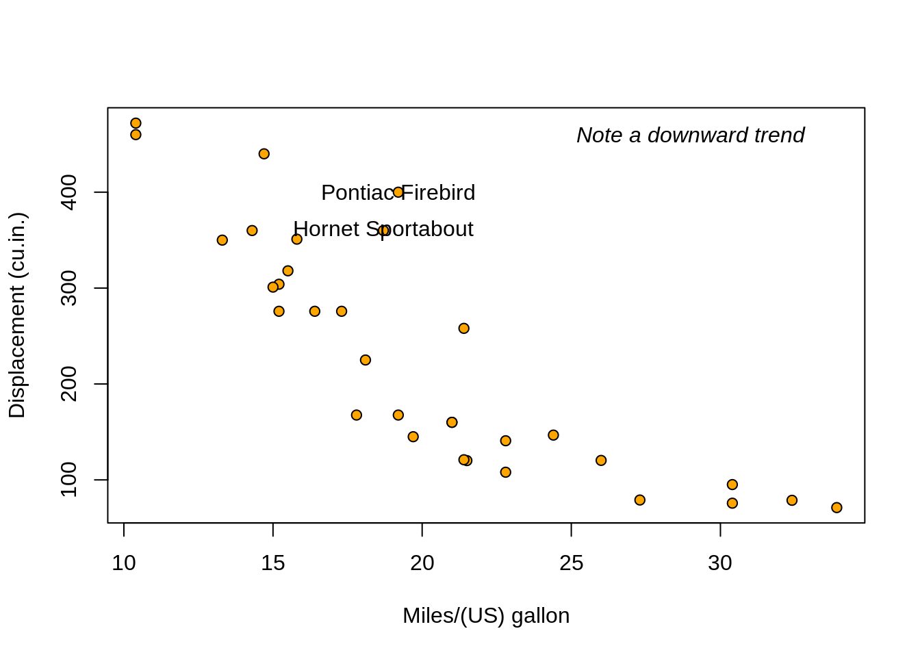
We can definitely improve the location of these labels. Let's add some offset to the x-axis. We can do this two ways:
- Literally add an offset to x, or
- Use the
adjargument.
Below is the example for option (1).
# Original chart
plot(mtcars$mpg, mtcars$disp, xlab='Miles/(US) gallon', ylab='Displacement (cu.in.)', pch=21, bg='orange')
# Text with some additional comments
text(x=29,y=460,'Note a downward trend', font=3)
# Label to some cars with an offset to x-axis
text(x=subset_mtcars$mpg+4.5,y=subset_mtcars$disp,labels=row.names(subset_mtcars))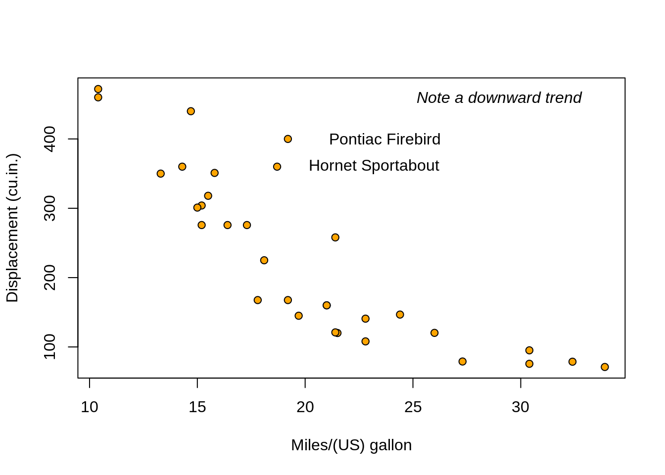
Below is the example for option (2).
# Original chart
plot(mtcars$mpg, mtcars$disp, xlab='Miles/(US) gallon', ylab='Displacement (cu.in.)', pch=21, bg='orange')
# Text with some additional comments
text(x=29,y=460,'Note a downward trend', font=3)
# Label to some cars
text(x=subset_mtcars$mpg,y=subset_mtcars$disp,labels=row.names(subset_mtcars), adj=-0.1)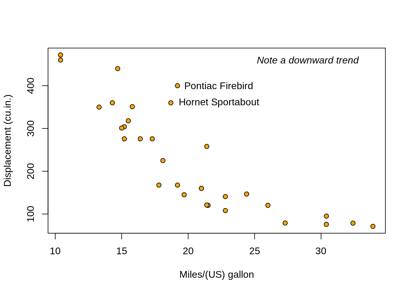
Could we decrease the size of the labels?
# Original chart
plot(mtcars$mpg, mtcars$disp, xlab='Miles/(US) gallon', ylab='Displacement (cu.in.)', pch=21, bg='orange')
# Text with some additional comments
text(x=29,y=460,'Note a downward trend', font=3)
# Label to some cars
text(x=subset_mtcars$mpg,y=subset_mtcars$disp,labels=row.names(subset_mtcars), adj=-0.1, cex=.8)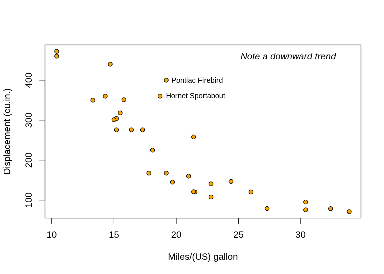
mtext
mtext is similar to the text function. However, it enables you to write in one of the four margins of the plot. Below is an example using the built-in mtcars dataset.
# Original chart
plot(mtcars$mpg, mtcars$disp, xlab='Miles/(US) gallon', ylab='Displacement (cu.in.)', pch=21, bg='orange', main='Motor trend car results')
# Adding text to the top margin:
mtext("Data from 1974 Motor Trend US magazine", font=3, cex=.7) # Recall that `cex` controls the font size.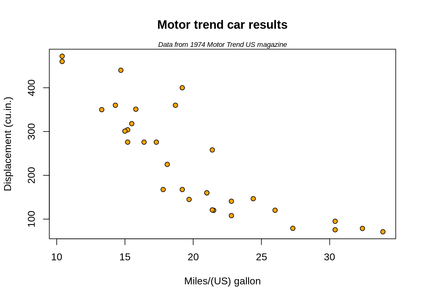
legend
The legend function enables us to add legends to plots. The example below uses the built-in dataset iris. The scatter plot below colors the data based on the flower's species.
# Original chart, colors are based on species
plot(iris$Sepal.Length, iris$Sepal.Width, xlab='Sepal length', ylab='Sepal width', pch=21, bg=iris$Species) 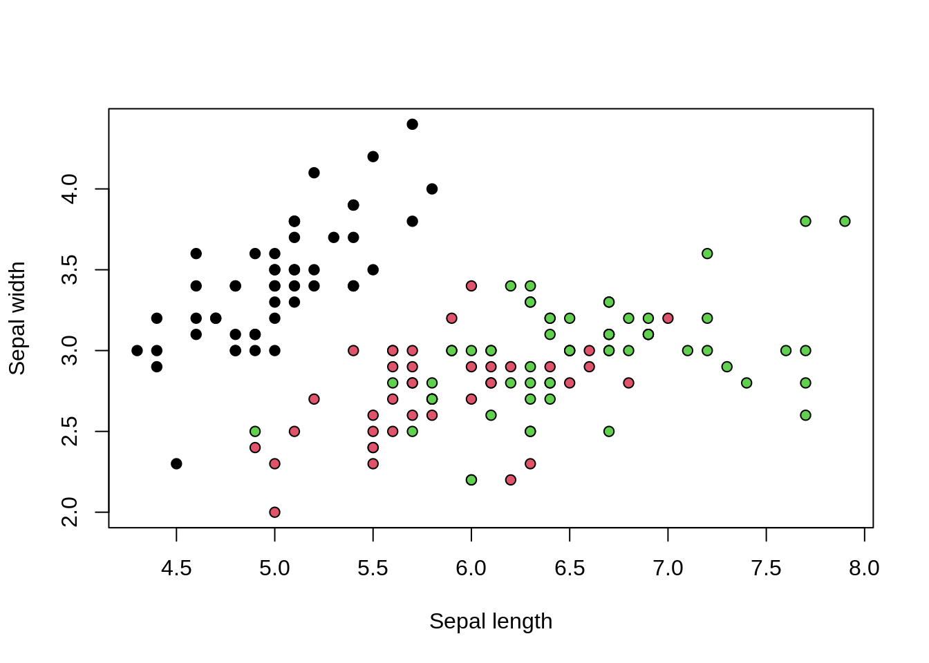
Let's create a legend for this plot to make it clear what the colors represent.
# Original chart, colors are based on species
plot(iris$Sepal.Length, iris$Sepal.Width, xlab='Sepal length', ylab='Sepal width', pch=21, bg=iris$Species)
# Adding a legend:
legend("topright", legend=unique(iris$Species), col=1:3, pc=20)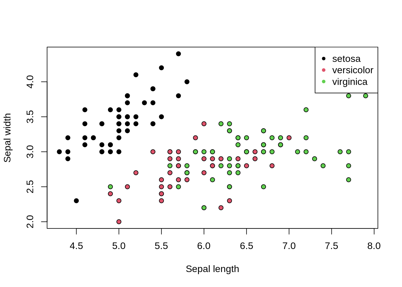
We can improve the look of the legend by making the points bigger, and removing the box.
# Original chart, colors are based on species
plot(iris$Sepal.Length, iris$Sepal.Width, xlab='Sepal length', ylab='Sepal width', pch=21, bg=iris$Species)
# Adding a legend:
legend("topright", legend=unique(iris$Species), col=1:3, pc=20,
pt.cex = 1.5, # changing just the point size
bty='n') # removing box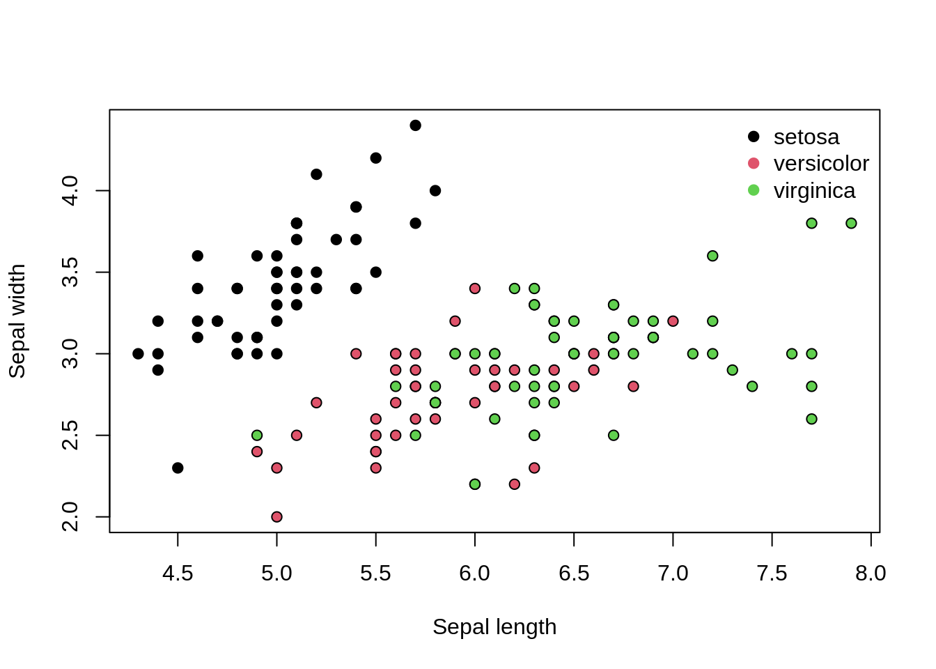
What if we made the legend's text smaller and italicized?
# Original chart, colors are based on species
plot(iris$Sepal.Length, iris$Sepal.Width, xlab='Sepal length', ylab='Sepal width', pch=21, bg=iris$Species)
# Adding a legend:
legend("topright", legend=unique(iris$Species), col=1:3, pc=20,
cex = .9, # text size
text.font=3, # italic text
pt.cex = 1.5, # changing just the point size
bty='n') # removing box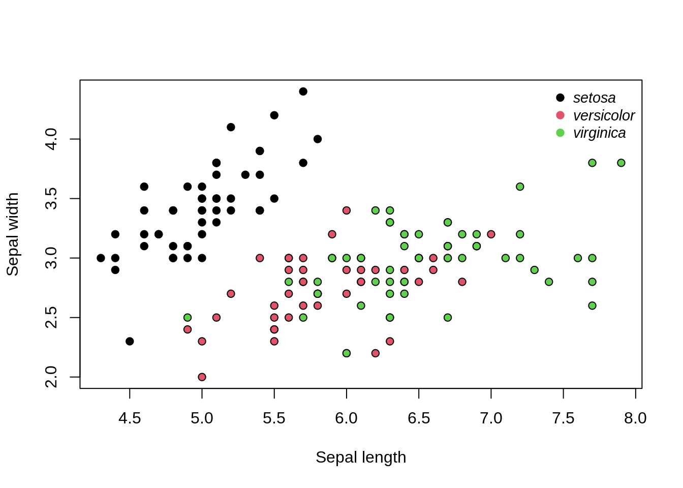
par
par allows us to set several graphical parameters. Among the many parameters that can be set, some of the most commonly used ones are mfrow, mfcol, mar, and oma. mfrow and mfcol enables us to create a layout for plots, so that we can include several graphs side by side. mar and oma set margins using the following form c(bottom, left, top, right). oma looks at outer margins.
Note that you can set several parameters all at once.
mfrow, mfcol
The example below uses the built-in data mtcars. mfrow and mfcol takes vector of the form c(nr, nc), where nr represents the number of rows and nc the number of columns.
par(mfrow=c(2,3)) # two rows, three columns
# Plot #1
plot(mtcars$mpg, mtcars$disp, xlab='Miles/(US) gallon', ylab='Displacement (cu.in.)', pch=21, bg='orange', main='Plot 1')
# Plot #2
boxplot(mtcars$wt, xlab='Weight (1000 lbs)', col='steelblue',main='Plot 2')
# Plot #3
barplot(table(mtcars$vs), col=c('tomato',"#23395b"), xlab='Engine', names.arg = c('V-shaped', 'Straight'), main='Plot 3')
# Plot #4
dotchart(mtcars$mpg, pch=21, bg="#43418A", xlim=c(10, 42), xlab='Miles/(US) gallon', main='Plot 4')
text(mtcars$mpg[c(1:2, 31:32)], c(1:2, 31:32), labels=row.names(mtcars)[c(1:2, 31:32)], adj = -.2, cex = .75, font=4)
# Plot #5
pie(table(mtcars$am), labels=c('Automatic', 'Manual'), main='Plot 5')
# Plot #6
boxplot(mtcars$hp ~mtcars$am, names=c("Automatic", "Manual"), xlab='Transmission', ylab='Horsepower', col=c("#ceb888","#03A696"), main='Plot 6')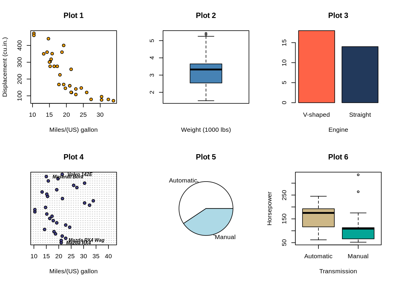
mar, oma
The example below uses the built-in data iris.
# Original plot
plot(iris$Sepal.Length, iris$Sepal.Width, xlab='Sepal length', ylab='Sepal width', pch=21, bg=iris$Species)
# Adding a legend:
legend("topright", legend=unique(iris$Species), col=1:3, pc=20,
cex = .9, # text size
text.font=3, # italic text
pt.cex = 1.5, # changing just the point size
bty='n') # removing box
Remove all margins.
par(mar=c(0,0,0,0))
# Original plot
plot(iris$Sepal.Length, iris$Sepal.Width, xlab='Sepal length', ylab='Sepal width', pch=21, bg=iris$Species)
# Adding a legend:
legend("topright", legend=unique(iris$Species), col=1:3, pc=20,
cex = .9, # text size
text.font=3, # italic text
pt.cex = 1.5, # changing just the point size
bty='n') # removing box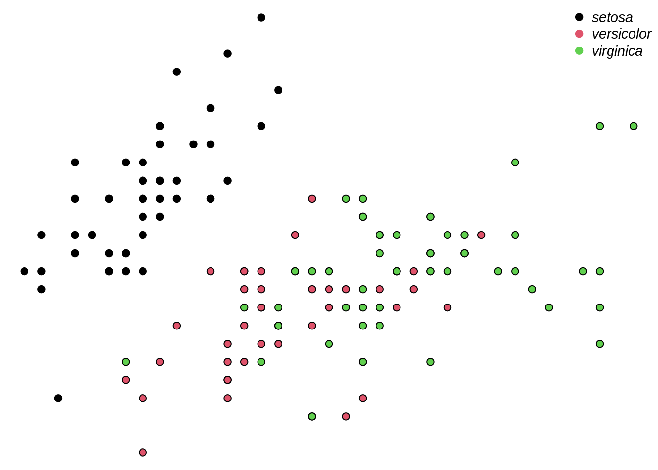
Add larger margins on the bottom and left side.
par(mar=c(4,6,2,2))
# Original plot
plot(iris$Sepal.Length, iris$Sepal.Width, xlab='Sepal length', ylab='Sepal width', pch=21, bg=iris$Species)
# Adding a legend:
legend("topright", legend=unique(iris$Species), col=1:3, pc=20,
cex = .9, # text size
text.font=3, # italic text
pt.cex = 1.5, # changing just the point size
bty='n') # removing box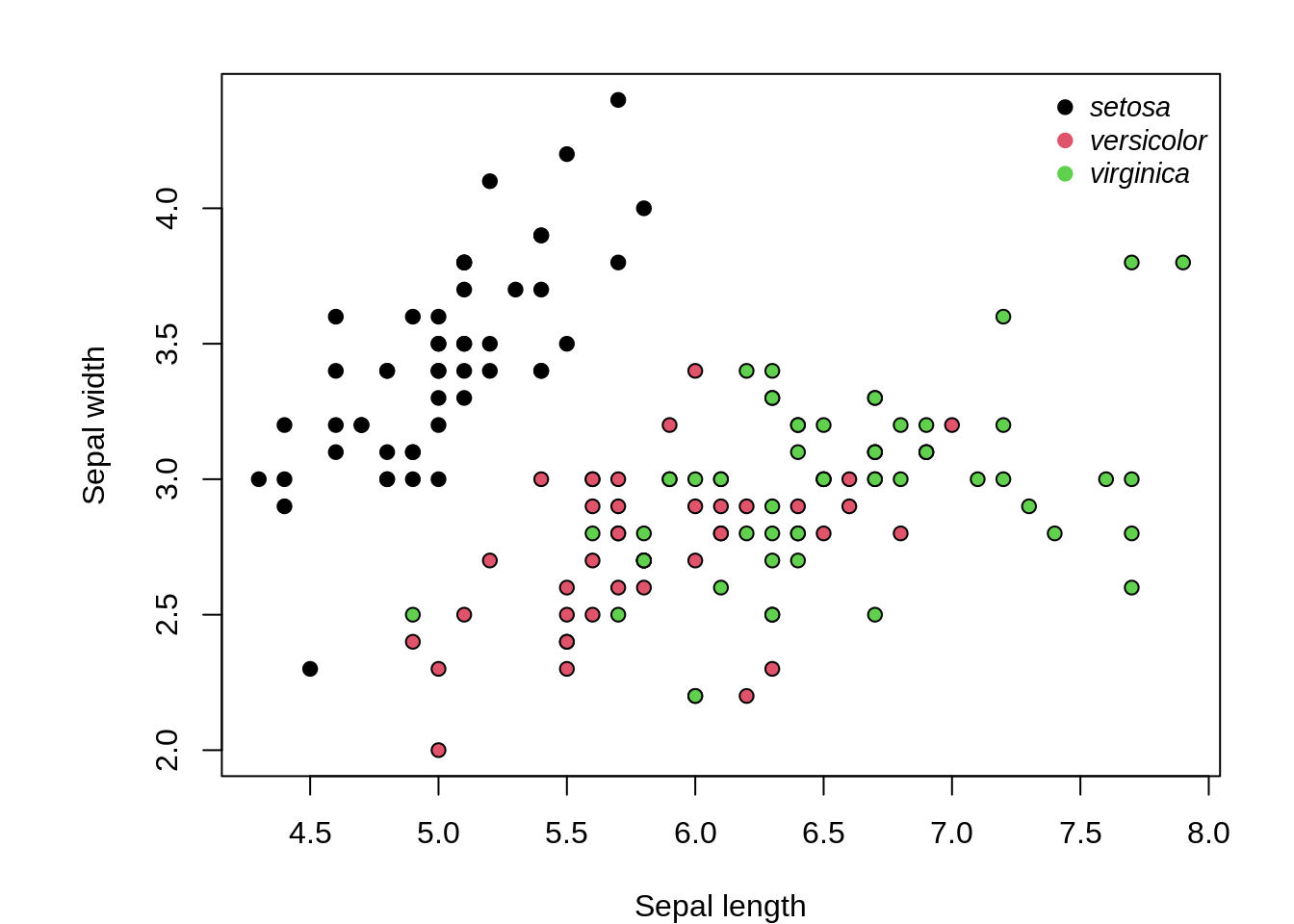
How do these margins look set on two plots side by side?
par(mar=c(4,6,2,2), mfrow=c(1,2))
# First plot
plot(iris$Sepal.Length, iris$Sepal.Width, xlab='Sepal length', ylab='Sepal width', pch=21, bg=iris$Species)
# Adding a legend:
legend("topright", legend=unique(iris$Species), col=1:3, pc=20,
cex = .9, # text size
text.font=3, # italic text
pt.cex = 1.5, # changing just the point size
bty='n') # removing box
# Second plot
plot(iris$Petal.Length, iris$Petal.Width, xlab='Petal length', ylab='Peta width', pch=21, bg=iris$Species)
# Adding a legend:
legend("bottomright", legend=unique(iris$Species), col=1:3, pc=20,
cex = .9, # text size
text.font=3, # italic text
pt.cex = 1.5, # changing just the point size
bty='n') # removing box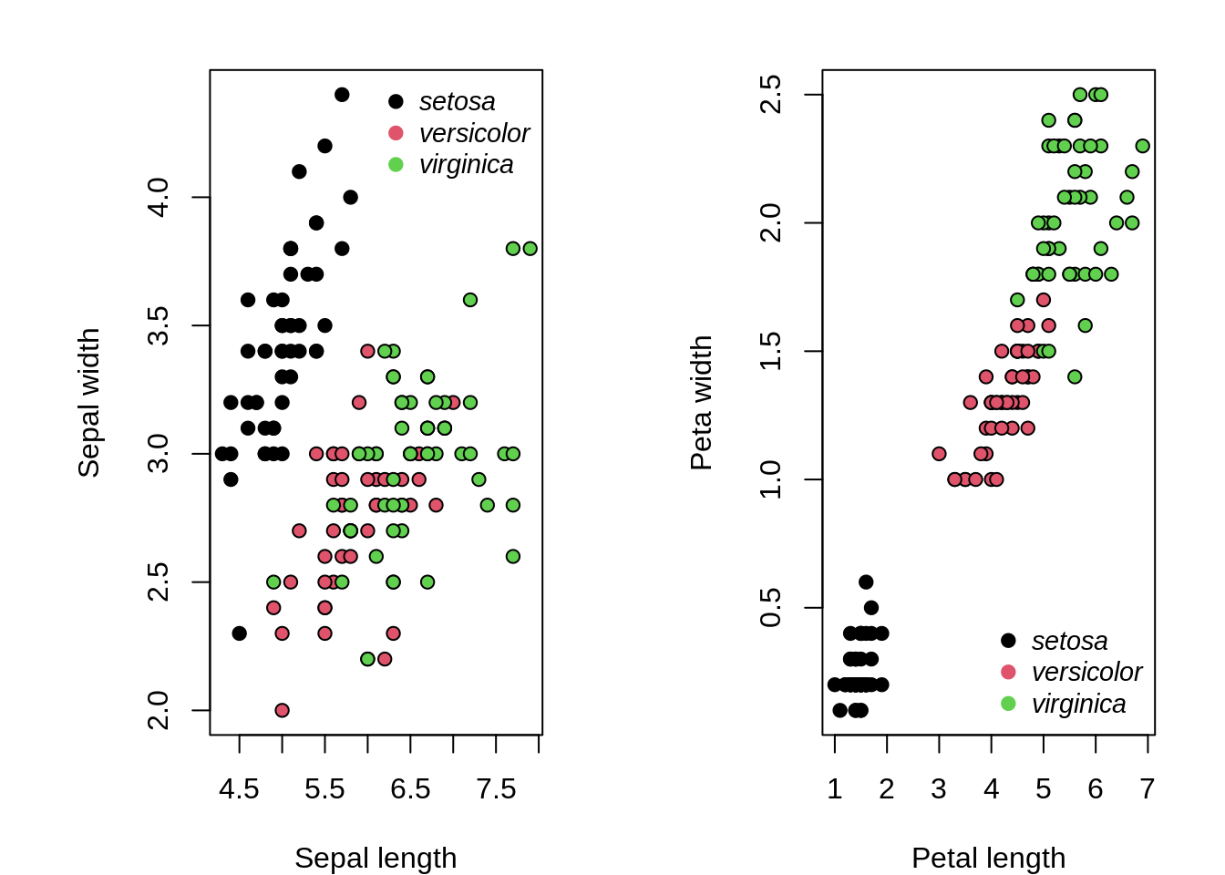
Doesn't look very good. Let's try setting smaller margins. Note that the default values for mar are mar=c(5.1, 4.1, 4.1, 2.1).
par(mar=c(4, 4, 2, 1), mfrow=c(1,2))
# First plot
plot(iris$Sepal.Length, iris$Sepal.Width, xlab='Sepal length', ylab='Sepal width', pch=21, bg=iris$Species)
# Adding a legend:
legend("topright", legend=unique(iris$Species), col=1:3, pc=20,
cex = .9, # text size
text.font=3, # italic text
pt.cex = 1.5, # changing just the point size
bty='n') # removing box
# Second plot
plot(iris$Petal.Length, iris$Petal.Width, xlab='Petal length', ylab='Peta width', pch=21, bg=iris$Species)
# Adding a legend:
legend("bottomright", legend=unique(iris$Species), col=1:3, pc=20,
cex = .9, # text size
text.font=3, # italic text
pt.cex = 1.5, # changing just the point size
bty='n') # removing box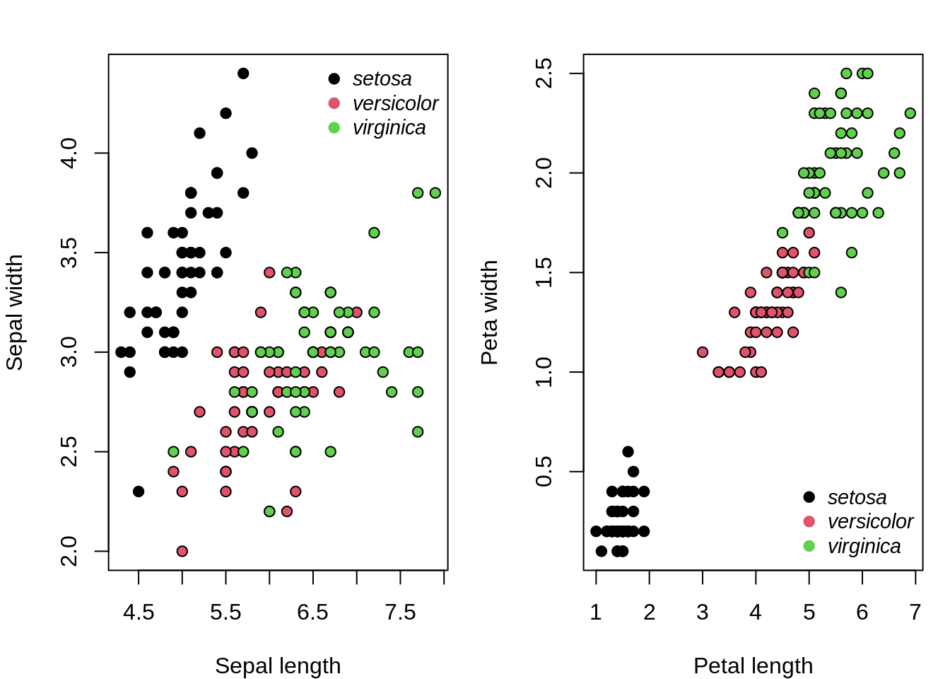
Perhaps we don't need two legends. How about we increase the margins (outer and usual) for top and bottom to include legend at the bottom, and a join title at the top?
par(mar=c(6, 4, 1, 1), mfrow=c(1,2), oma=c(2,0,3,0))
# First plot
plot(iris$Sepal.Length, iris$Sepal.Width, xlab='Sepal length', ylab='Sepal width', pch=21, bg=iris$Species)
# Adding a legend
legend("bottom",legend=unique(iris$Species), col=1:3, pc=20,
cex = .8, # text size
text.font=3, # italic text
pt.cex = 1.5, # changing just the point size
bty='n',# removing box
xpd = TRUE, horiz = TRUE, # make legend horizontal
inset=c(2,-0.50)) # changes to x and y positions
# Second plot
plot(iris$Petal.Length, iris$Petal.Width, xlab='Petal length', ylab='Peta width', pch=21, bg=iris$Species)
# Joint title
mtext("Results for 3 species of iris flowers", outer=TRUE, font=2)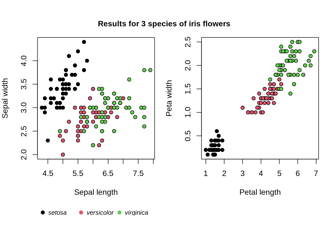
facet_grid
facet_grid is a function that allows you to easily create duplicate plots of different groupings of data. For example, let's say we have the following plot:
g <- ggplot(iris, aes(x=Petal.Length, y=Petal.Width, col=Species)) + geom_point(alpha=.33)
g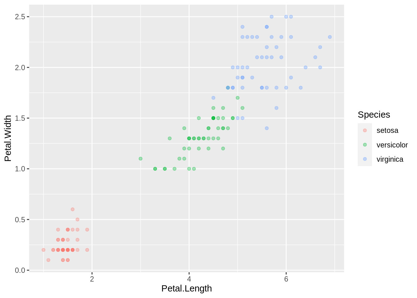
Here, we can see the Petal.Width on the y-axis and Petal.Length on the x-axis for each of the 3 species of plant. It's not a horrible plot, however, with facet_grid, we have some simple ways to visualize the data. For example, you could imagine a dataset where the divide between virginica and versicolor is less clear. In this situation, perhaps breaking the plot to be side-by-side would be best:
g <- ggplot(iris, aes(x=Petal.Length, y=Petal.Width, col=Species)) + geom_point(alpha=.33)
g + facet_grid(Species ~ .)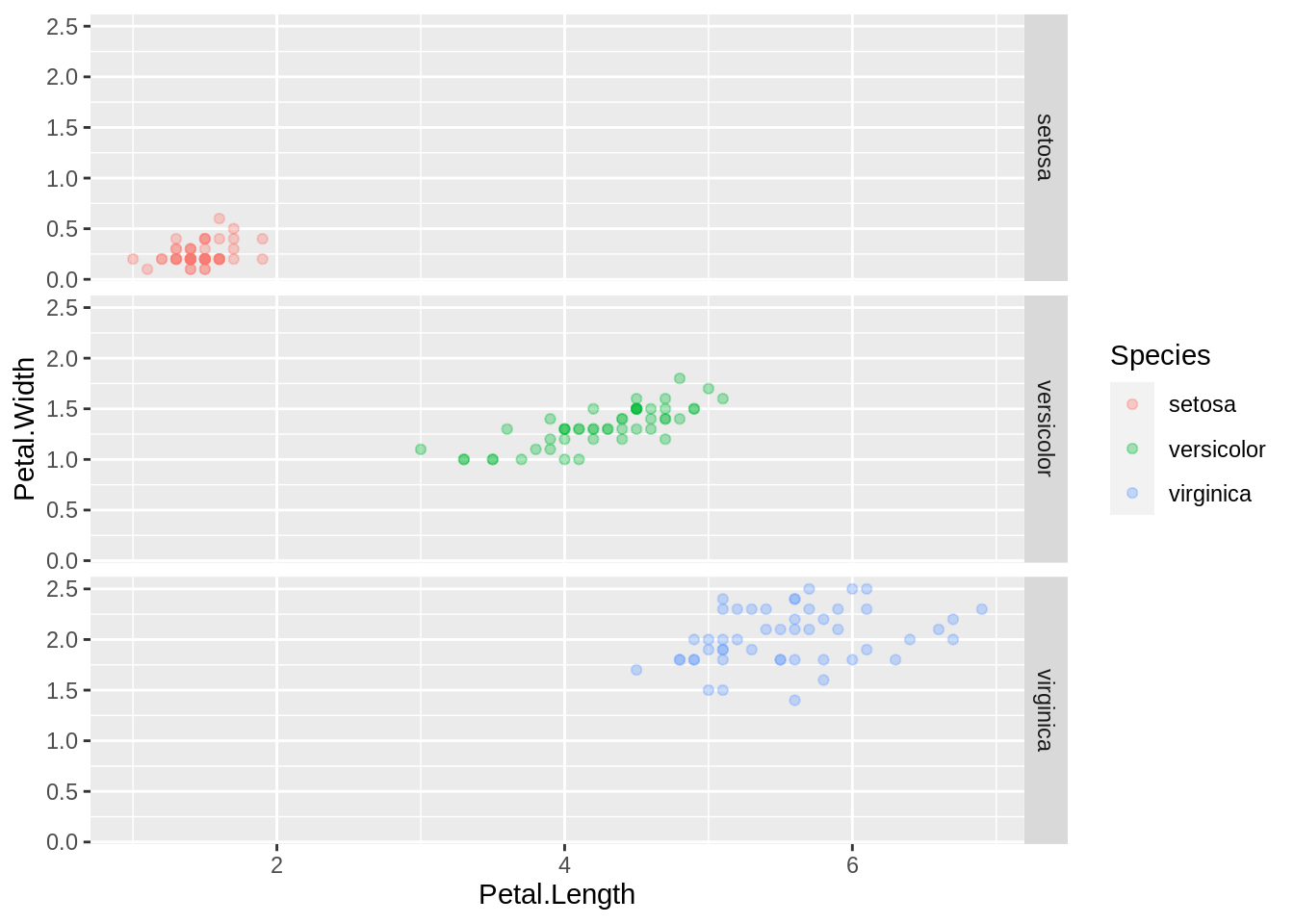
Here, on the lefthand side of ~, we have the variable to split the rows by. On the righthand side we put . which is where we could put the variable where we would split the columns by, but instead we put . which just means we aren't splitting by columns. We could swap the positions to split by columns instead:
g <- ggplot(iris, aes(x=Petal.Length, y=Petal.Width, col=Species)) + geom_point(alpha=.33)
g + facet_grid(. ~ Species)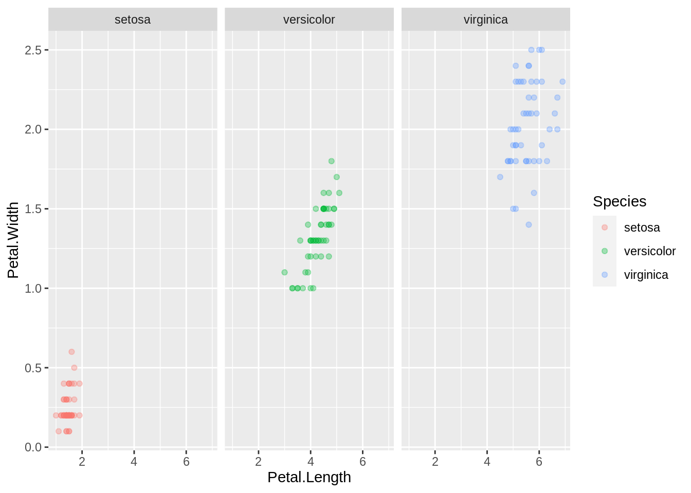
That is an incredibly telling plot without very much work at all. Let's take a look at another built-in dataset to see an even more complicated plot.
Let's say we wanted to analyze the city vs highway miles per gallon, by manufacturers:
g <- ggplot(mpg, aes(x=cty, y=hwy, col=manufacturer)) + geom_point(alpha=.33)
g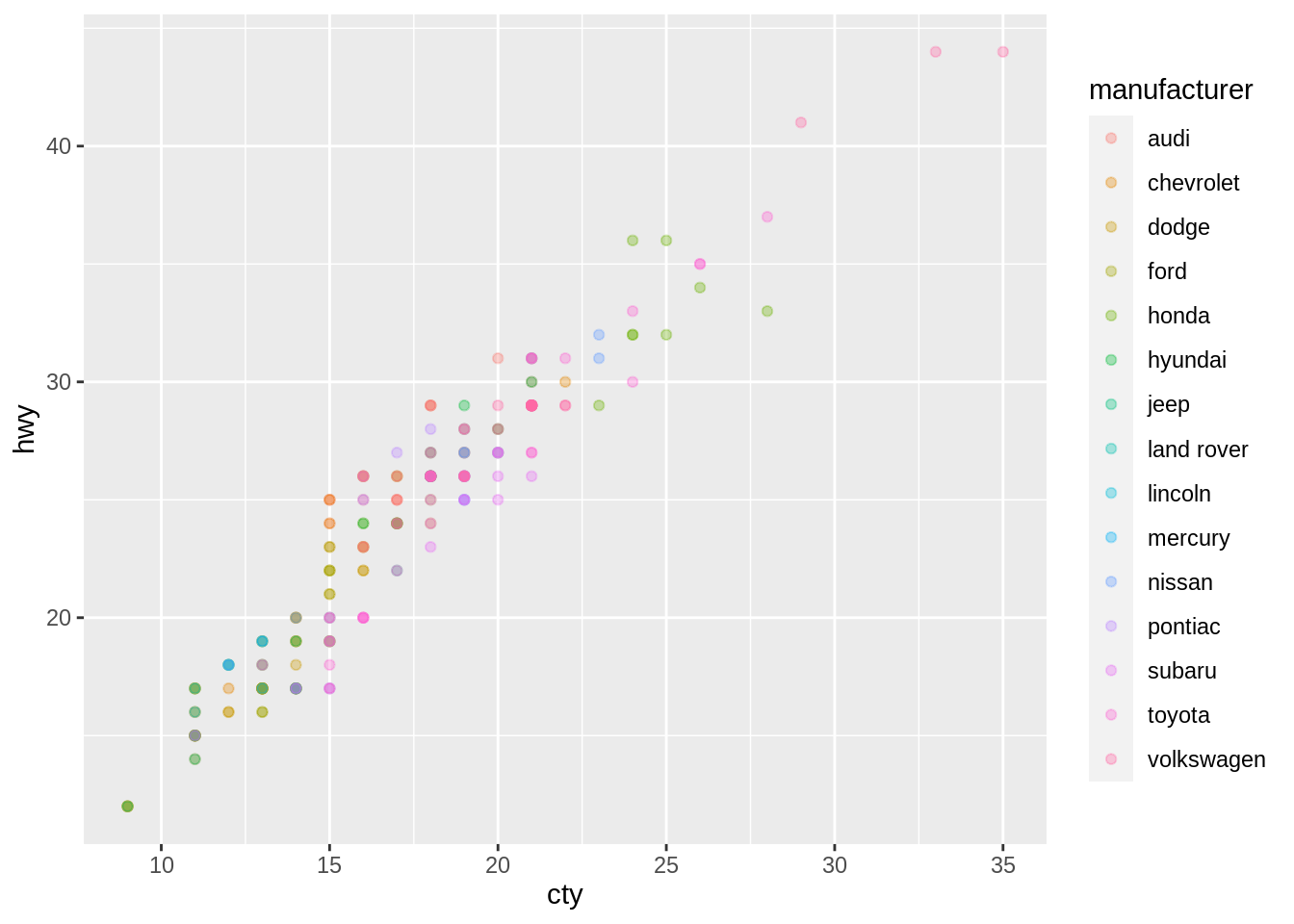
As you can see, it becomes more clear why a function like facet_grid can come in handy. Let's fix this up a little:
g <- ggplot(mpg, aes(x=cty, y=hwy, col=manufacturer)) + geom_point(alpha=.33)
g + facet_grid(. ~ manufacturer)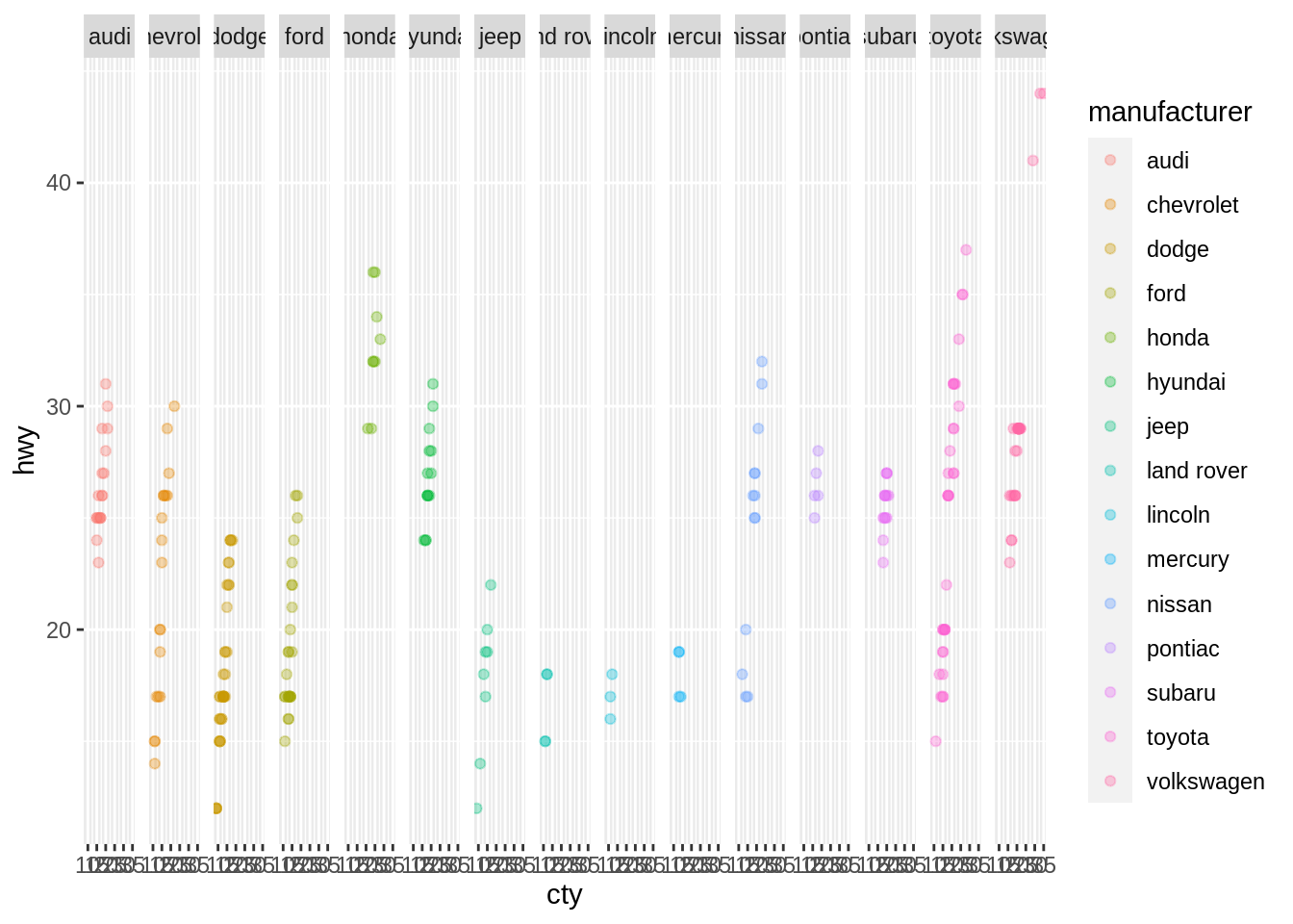
Well, that is not particularly useful. This is an example where facet_wrap may come in handy.
facet_wrap
facet_wrap is very similar to facet_grid, with 2 primary differences.
- Groupings of factors with no data are not displayed using
facet_wrap. - The columns and rows in
facet_gridare strictly defined by the groupings,facet_wrapjust considers each grouping containing data a factor to be displayed in a chart.
So for example, in our last example in the facet_grid section, we try to display city vs highway miles per gallon by manufacturer. The resulting graphic was extremely crowded and not useful. Using facet_wrap, each manufacturer gets its own plot with city mpg on the x-axis and highway mpg on the y-axis:
g <- ggplot(mpg, aes(x=cty, y=hwy, col=manufacturer)) + geom_point(alpha=.33)
g + facet_wrap(. ~ manufacturer, ncol=4)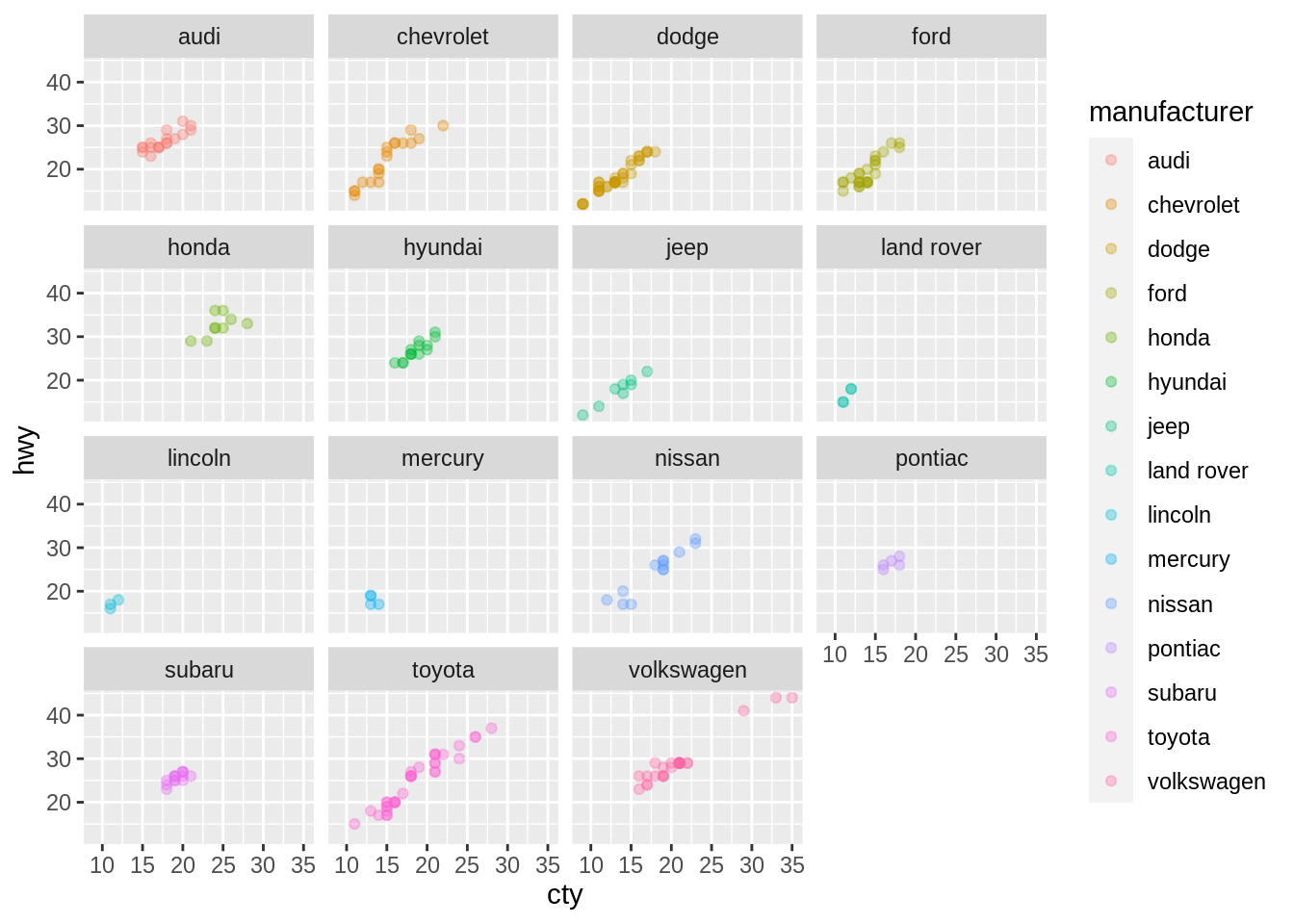
Here, we specified that we want 4 columns. facet_wrap fills the columns one-by-one until there are no remaining plots to plot. We could easily change this. For example, we have 15 plots, if we wanted to waste less space we could specify 3 columns and 5 rows:
g <- ggplot(mpg, aes(x=cty, y=hwy, col=manufacturer)) + geom_point(alpha=.33)
g + facet_wrap(. ~ manufacturer, ncol=3, nrow=5)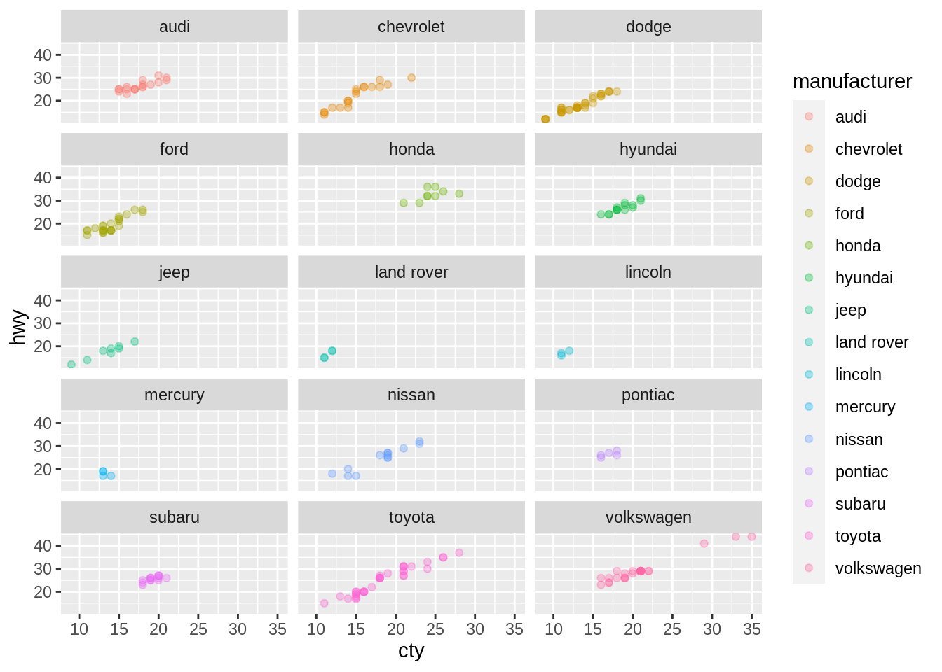
Of course, if you just specified 3 columns, facet_wrap would continue to add plots, one-by-one, until all of the plots are displayed, so we would end up with 5 rows without specifying that we want 5 rows:
g <- ggplot(mpg, aes(x=cty, y=hwy, col=manufacturer)) + geom_point(alpha=.33)
g + facet_wrap(. ~ manufacturer, ncol=3)
plot_usmap
usmap is a package dedicated to get maps of the US by varying region types. Includes the plot_usmap function which allows you do easily plot state or region level data on top of a map.
First, load up the package:
library(usmap)You can generate the default map pretty easily.
plot_usmap("states", labels=T)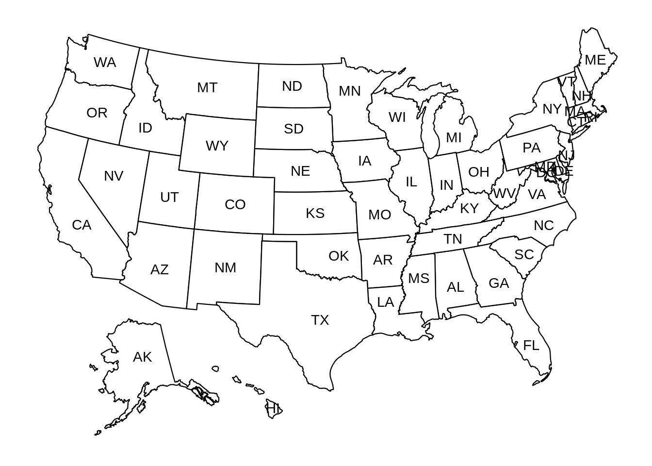
The first argument, regions can be "states", "state", "counties", or "county". You can switch the borders by changing this argument.
plot_usmap("counties", labels=T)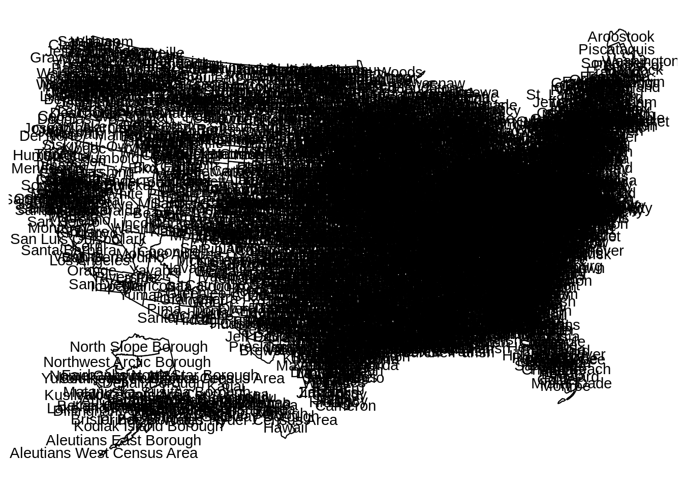 As you can see, adding the labels in this case, obfuscates our map.
plot_usmap("counties", labels=F) If we wanted to zoom in on a state, this is easy to do.
plot_usmap("counties", include=c("IN")) Of course, you can still just zoom in on a group of states, you don't have to show the county lines.
plot_usmap("states", labels=T, include=c("IL", "MI", "IN", "OH"))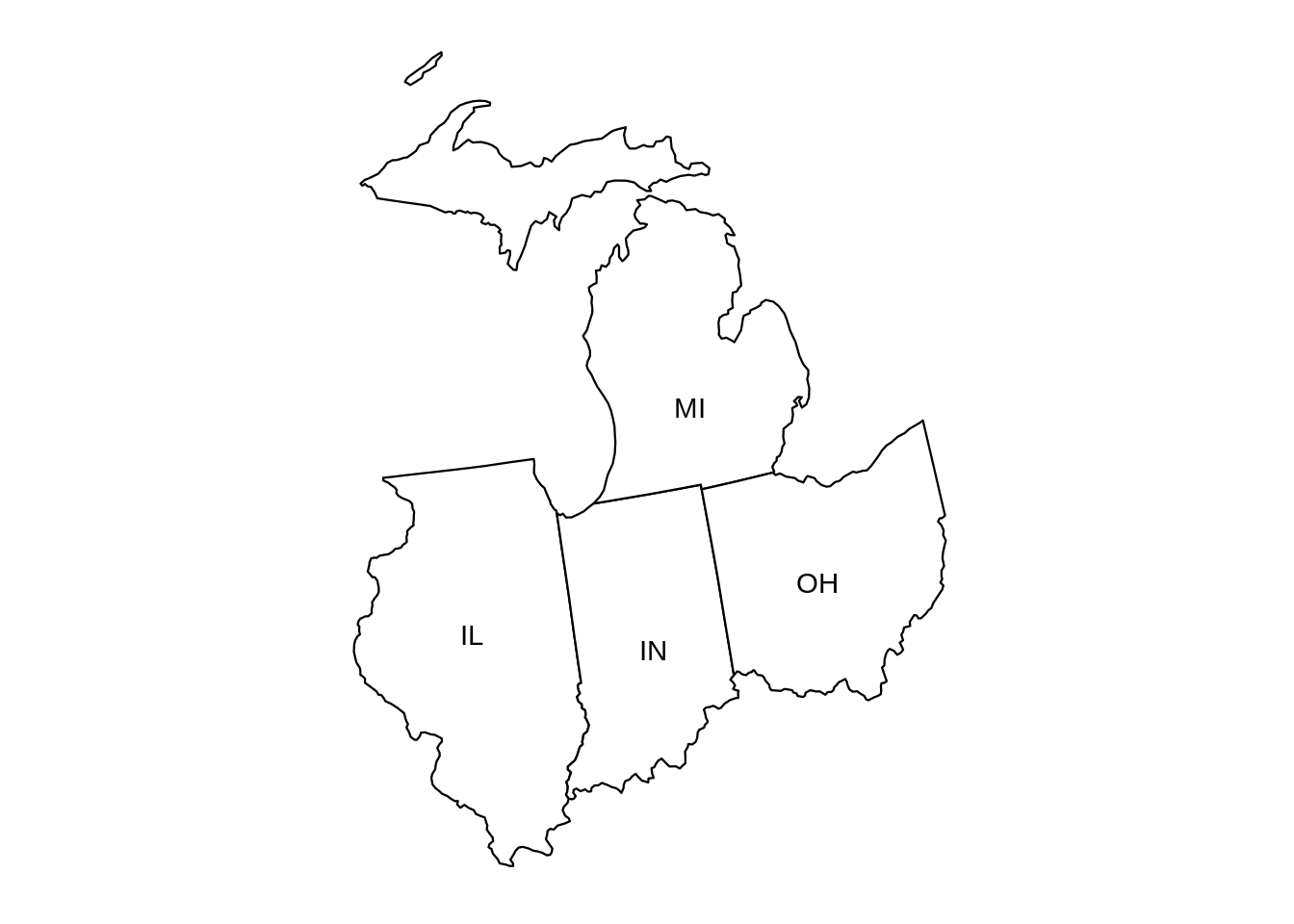 Pretty incredible. You can change the label colors using the
 label_color argument.
plot_usmap("states", labels=T, include=c("IL", "MI", "IN", "OH"), label_color="gold")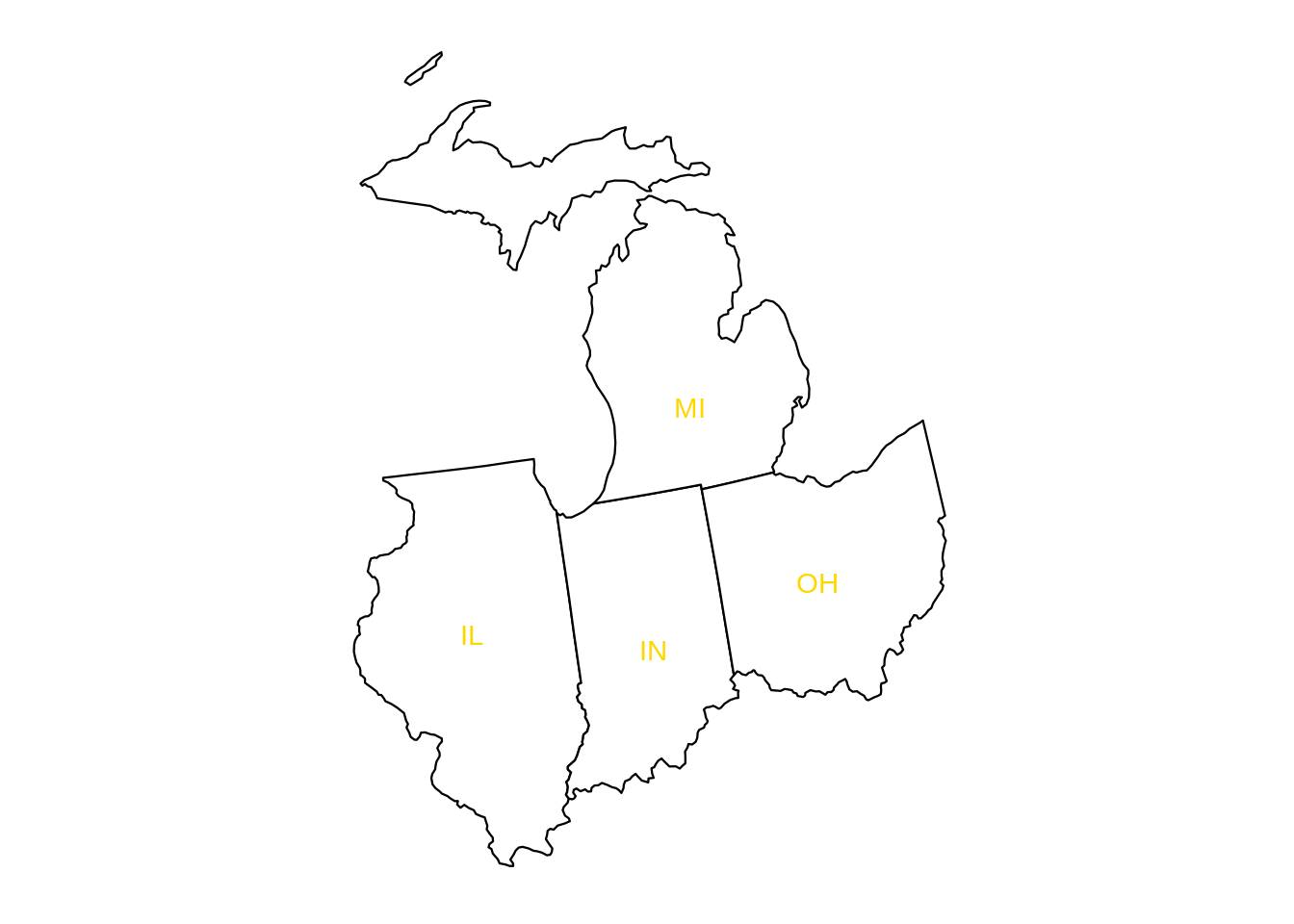 You can even have different colors for each of the states.
plot_usmap("states", labels=T, include=c("IL", "MI", "IN", "OH"), label_color=c("blue", "green", "gold", "tomato")) Similarly, you can control the fill color using the
 fill argument.
plot_usmap("states", labels=T, include=c("IL", "MI", "IN", "OH"), label_color=c("blue", "green", "gold", "tomato"), fill="grey") You can control the border color using the
 color argument.
plot_usmap("states", labels=T, include=c("IL", "MI", "IN", "OH"), label_color=c("blue", "green", "gold", "tomato"), fill="grey", color="white") We can control the border width with the
 size argument as well.
plot_usmap("states", labels=T, include=c("IL", "MI", "IN", "OH"), label_color=c("blue", "green", "gold", "tomato"), fill="grey", color="white", size=2) Of course, it is important to be able to utilize a dataset with
 plot_usmap. To do so you must use the data and values arguments.
The data argument expects a data.frame with at least two columns. One column to indicate which state or county, and another to indicate the associated values (whatever they may be). The column indicating the state or value must be named either fips or state. The other column can be anything as long as you use the values argument to specify the name.
myDF <- data.frame(state=state.abb, val=datasets::state.area)
head(myDF)## state val
## 1 AL 51609
## 2 AK 589757
## 3 AZ 113909
## 4 AR 53104
## 5 CA 158693
## 6 CO 104247plot_usmap(data=myDF, values="val", labels=T, include=c("IL", "MI", "IN", "OH"))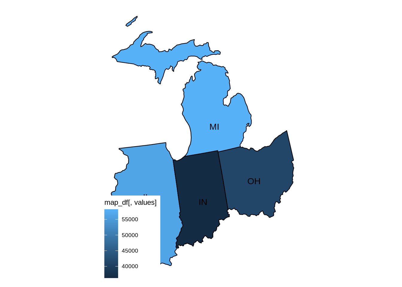 To move the legend out of the way, you can use
 theme from ggplot2.
library(ggplot2)
plot_usmap(data=myDF, values="val", labels=T, include=c("IL", "MI", "IN", "OH")) +
theme(legend.position = "right")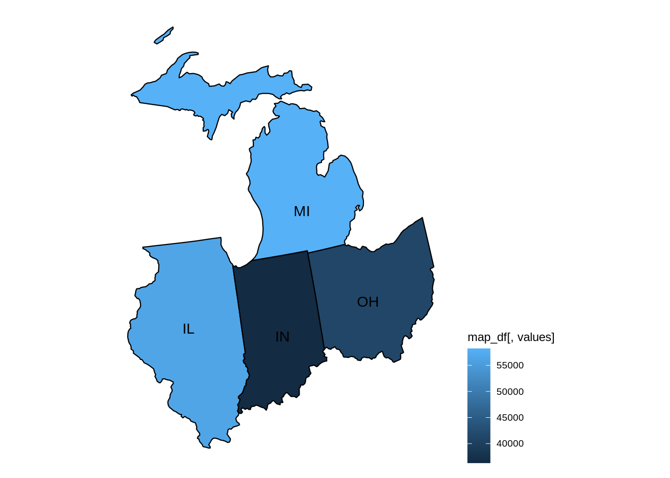 If we wanted to change the colors and way the shading works, we can use
 scale_fill_continous from ggplot2.
library(ggplot2)
plot_usmap(data=myDF, values="val", labels=T, include=c("IL", "MI", "IN", "OH")) +
theme(legend.position = "right") +
scale_fill_continuous(low="white", high="navy")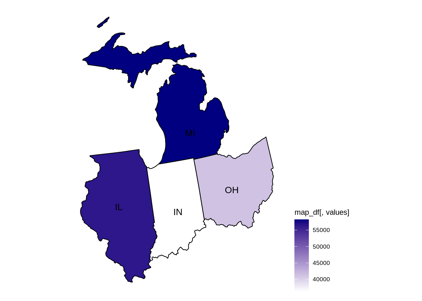 It would probably look better if we had more than 4 points. Let's try with the entire US.
library(ggplot2)
plot_usmap(data=myDF, values="val", labels=T) +
theme(legend.position = "right") +
scale_fill_continuous(low="white", high="navy")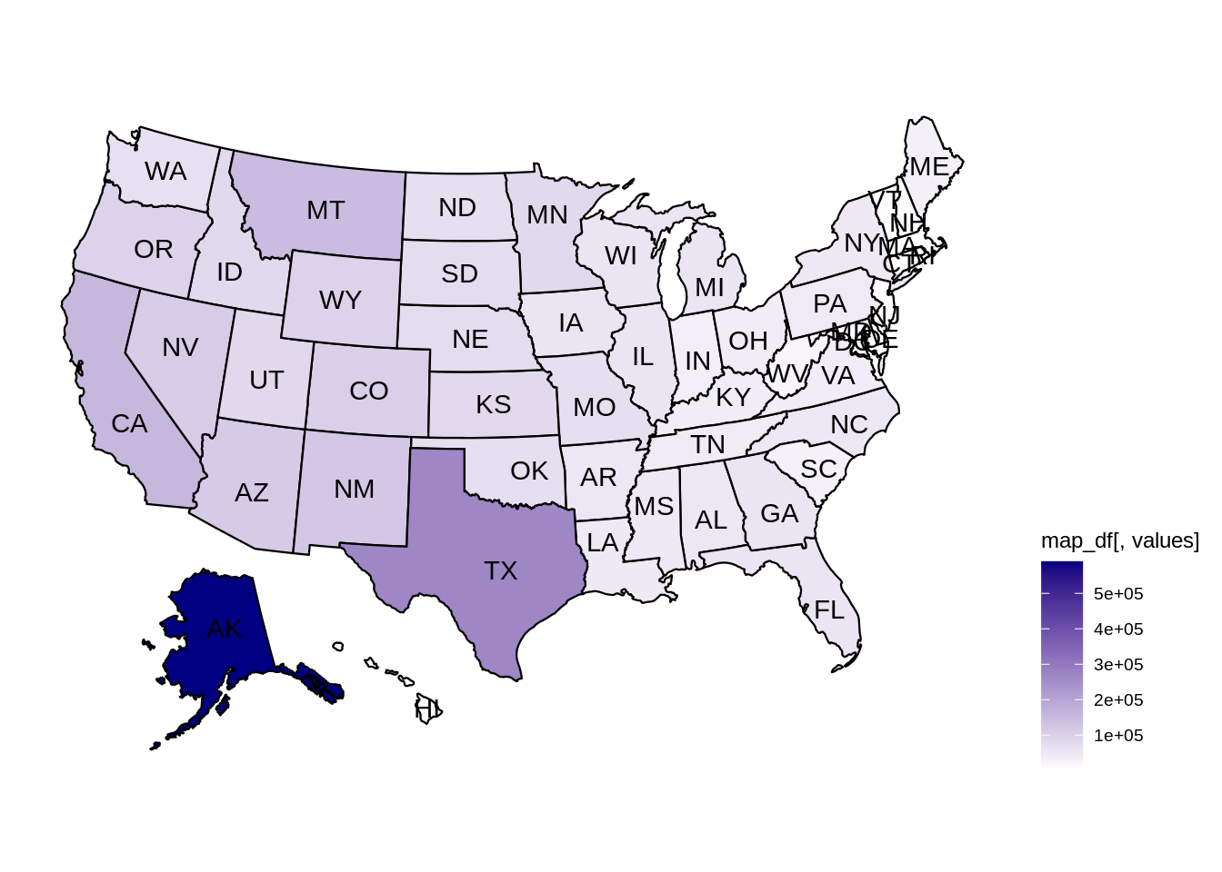 It really puts AK's area into perspective! How about if we remove AK using the
 exclude argument?
library(ggplot2)
plot_usmap(data=myDF, values="val", labels=T, exclude=c("AK")) +
theme(legend.position = "right") +
scale_fill_continuous(low="white", high="navy")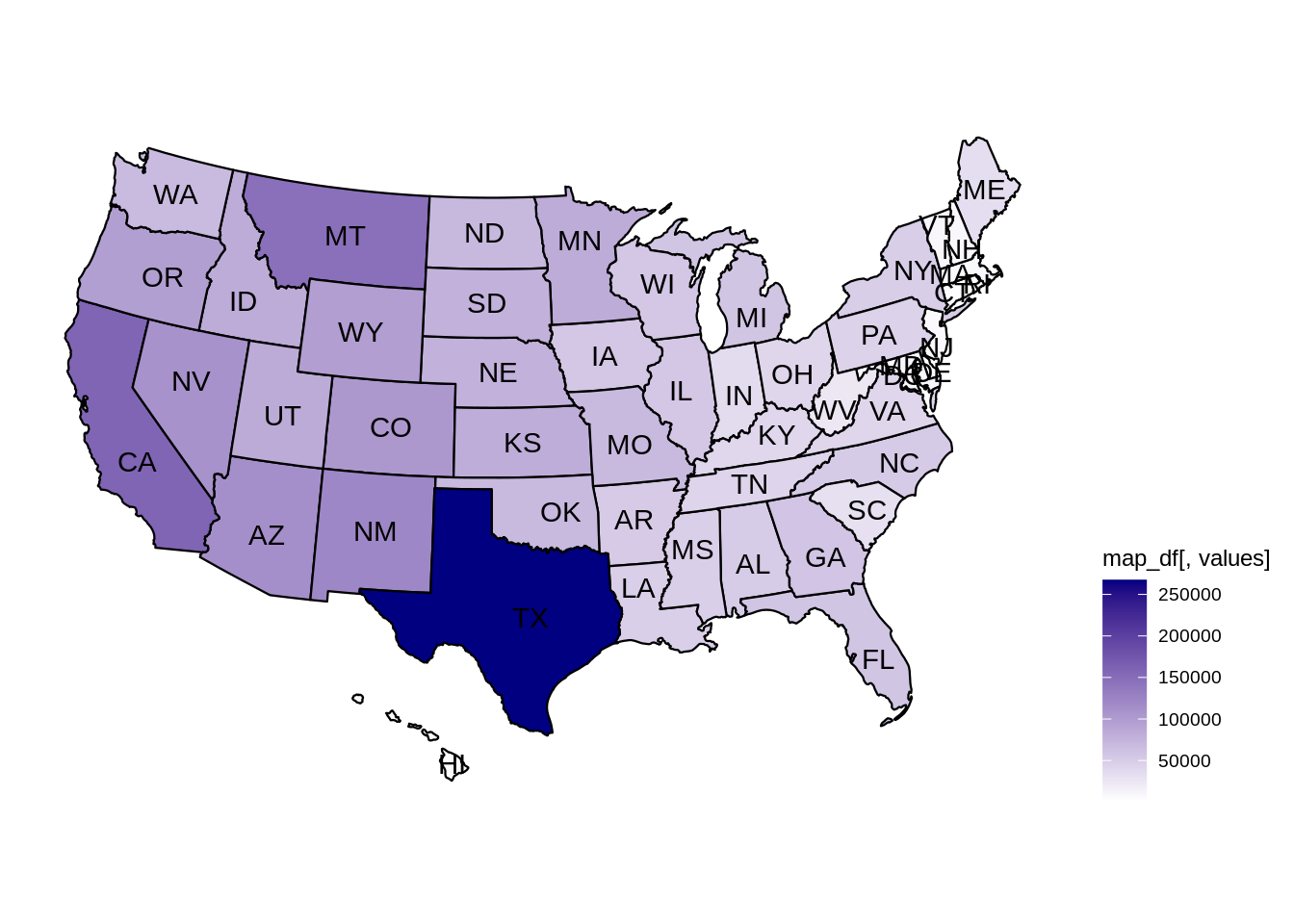 Note that if the
 regions argument is "state" or "states", either the state name, abbreviation, or fips code would work to identify the state. The full 5-digit fips code is required to identify counties, however. To get a fips code for a certain county, you can do the following.
usmap::fips(state = "IN", county="Tippecanoe")## [1] "18157"Note that the first 2 digits of the 5 digit fips code is the state fips code.
usmap::fips(state = "IN")## [1] "18"What if we wanted to show area by the percentage of area that the state represents? First we would need to calculate it.
myDF$percent_area <- myDF$val/sum(myDF$val)library(ggplot2)
plot_usmap(data=myDF, values="percent_area", labels=T) +
theme(legend.position = "right") +
scale_fill_continuous(low="white", high="navy")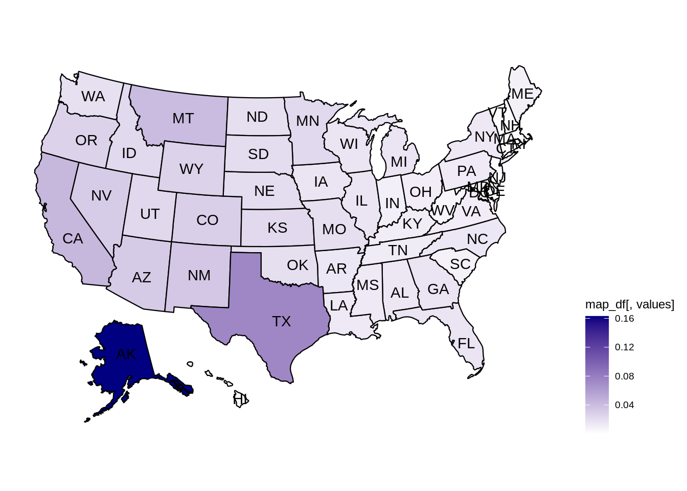 After that, we can use the
 scales packages to fix the legend up.
library(ggplot2)
plot_usmap(data=myDF, values="percent_area", labels=T) +
theme(legend.position = "right") +
scale_fill_continuous(low="white", high="navy", name="Percent of US area", label=scales::percent)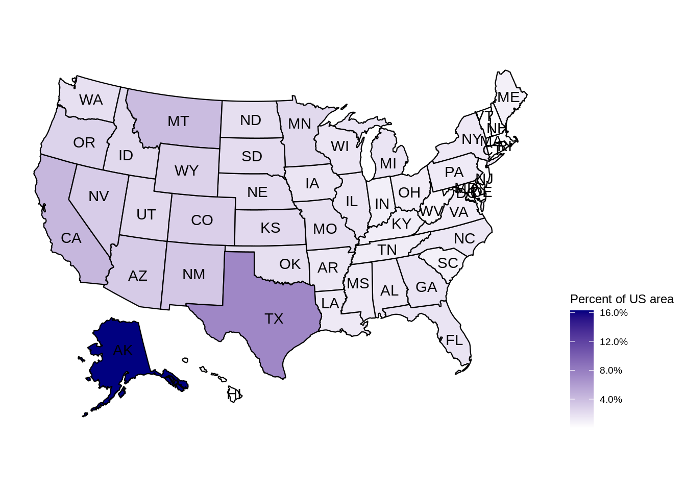 If you were working with data that would be better represented by dollars instead of percentages, you could simply change the
 label argument to scales::dollars.
Resources
A page with some code examples and output using usmap.
A page with some code examples and output using usmap. A little bit more in depth.
ggplot
The "gg" in ggplot stands for Grammar of Graphics. Essentially, it is a way of thinking about graphics as a collection of components that make up a plot.
ggplot additively builds a plot by adding component after component. See the plots in the plotting section to see examples using ggplot (following the base R equivalents).
ggmap
ggmap is an excellent package that provides a suite of functions that, among other things, allows you to map spatial data on top of static maps.
Important note: You must set up billing in order to use Google's APIs.
Getting started
To install ggmap, simply run install.packages("ggmap"). To load the library, run library(ggmap). When first using this package, you may notice you need an API key to get access to certain functionality. Follow the directions here to get an API key. It should looks somethings like: mQkzTpiaLYjPqXQBotesgif3EfGL2dbrNVOrogg.
Once you've acquired the API key, you have two options:
- Register
ggmapwith Google for the current session:
library(ggmap)
register_google(key="mQkzTpiaLYjPqXQBotesgif3EfGL2dbrNVOrogg")- Register
ggmapwith Google, persistently through sessions:
library(ggmap)
register_google(key="mQkzTpiaLYjPqXQBotesgif3EfGL2dbrNVOrogg", write=TRUE)Note that if you choose option (2), your API key will be saved within your ~/.Renviron.
Examples
How do I get a map of West Lafayette?
Click here for solution
map <- get_map(location="West Lafayette")
ggmap(map)How do I zoom in and out on a map of West Lafayette?
Click here for solution
# zoom way out
map <- get_map(location="West Lafayette", zoom=1)
ggmap(map)
# zoom in
map <- get_map(location="West Lafayette", zoom=12)
ggmap(map)How do I add Latitude and Longitude points to a map of Purdue University?
Click here for solution
points_to_add <- data.frame(latitude=c(40.433663, 40.432104, 40.428486), longitude=c(-86.916584, -86.919610, -86.920866))
map <- get_map(location="Purdue University", zoom=14)
ggmap(map) + geom_point(data = points_to_add, aes(x = longitude, y = latitude))leaflet
leaflet is a popular JavaScript library to create interactive maps. The leaflet R package makes it easy to create incredible interactive maps.
Examples
How do I plot some longitude and latitude points on an interactive map?
Click here for solution
library(leaflet)
points_to_plot <- data.frame(latitude=c(40.433663, 40.432104, 40.428486), longitude=c(-86.916584, -86.919610, -86.920866))
map <- leaflet()
map <- addTiles(map)
map <- addCircles(map, lng=points_to_plot$longitude, lat=points_to_plot$latitude)
map
# or another way with magrittr
library(magrittr)
leaflet(points_to_plot) %>% addTiles() %>% addCircles(lng=~longitude, lat=~latitude)magrittr is a package that adds the %>% and `%<% operators which allow you to pipe the output of R code to more R code, much like piping in bash. You can read more about it here.
RMarkdown
To install RMarkdown simply run the following:
install.packages("rmarkdown")Projects in The Data Mine are all written in RMarkdown. You can download the RMarkdown file by clicking on the link at the top of each project page. Each file should end in the ".Rmd" which is the file extension commonly associated with RMarkdown files.
You can find an exemplary RMarkdown file here:
https://raw.githubusercontent.com/TheDataMine/the-examples-book/master/files/rmarkdown.Rmd
If you open this file in RStudio, and click on the "Knit" button in the upper left hand corner of IDE, you will get the resulting HTML file. Open this file in the web browser of your choice and compare and contrast the syntax in the rmarkdown.Rmd file and resulting output. Play around with the file, make modifications, and re-knit to gain a better understanding of the syntax. Note that similar input/output examples are shown in the RMarkdown Cheatsheet.
Code chunks
Code chunks are sections within an RMarkdown file where you can write, display, and optionally evaluate code from a variety of languages:
## [1] "awk" "bash" "coffee" "gawk" "groovy"
## [6] "haskell" "lein" "mysql" "node" "octave"
## [11] "perl" "psql" "Rscript" "ruby" "sas"
## [16] "scala" "sed" "sh" "stata" "zsh"
## [21] "highlight" "Rcpp" "tikz" "dot" "c"
## [26] "cc" "fortran" "fortran95" "asy" "cat"
## [31] "asis" "stan" "block" "block2" "js"
## [36] "css" "sql" "go" "python" "julia"
## [41] "sass" "scss" "theorem" "lemma" "corollary"
## [46] "proposition" "conjecture" "definition" "example" "exercise"
## [51] "proof" "remark" "solution"The syntax is simple:
```{language, options...}
code here...
```For example:
```{r, echo=TRUE}
my_variable <- c(1,2,3)
my_variable
```Which will render like:
my_variable <- c(1,2,3)
my_variable## [1] 1 2 3You can find a list of chunk options here.
How do I run a code chunk but not display the code above the results?
Click here for solution
```{r, echo=FALSE}
my_variable <- c(1,2,3)
my_variable
```How do I include a code chunk without evaluating the code itself?
Click here for solution
```{r, eval=FALSE}
my_variable <- c(1,2,3)
my_variable
```How do I prevent warning messages from being displayed?
Click here for solution
```{r, warning=FALSE}
my_variable <- c(1,2,3)
my_variable
```How do I prevent error messages from being displayed?
Click here for solution
```{r, error=FALSE}
my_variable <- c(1,2,3)
my_variable
```How do I run a code chunk, but not include the chunk in the final output?
Click here for solution
```{r, include=FALSE}
my_variable <- c(1,2,3)
my_variable
```How do I render a figure from a chunk?
Click here for solution
```{r}
my_variable <- c(1,2,3)
plot(my_variable)
```How do I create a set of slides using RMarkdown?
Click here for solution
Please see the example Rmarkdown file here.
You can change the slide format by changing the yaml header to any of: ioslides_presentation, slidy_presentation, or beamer_presentation.
By default all first and second level headers (# and ##, respectively) will create a new slide. To manually create a new slide, you can use ***.
Resources
An excellent quick reference for RMarkdown syntax.
A thorough reference manual showing markdown input and expected output. Gives descriptions of the various chunk options, as well as output options.
A set of lessons detailing the ins and outs of RMarkdown.
RMarkdown uses Markdown syntax for its text. This is a good, interactive tutorial to learn the basics of Markdown. This tutorial is available in multiple languages.
This gallery highlights a variety of reproducible and interactive RMarkdown documents. An excellent resource to see the power of RMarkdown.
This is a chapter from Hadley Wickham's excellent R for Data Science book that details important parts of RMarkdown.
This is a nice article that introduces RMarkdown, and guides the user through creating their own interactive document using RMarkdown in RStudio.
This is another good resource that introduces RMarkdown. Plenty of helpful pictures and screenshots.
Tidyverse
piping
Much like the | operator in bash, the %>% operator in R pipes the output from the first expression to the second. For example, instead of:
sum(c(1,2,3))## [1] 6One can use %>%:
c(1,2,3) %>% sum()## [1] 6It is extremely common practice in the tidyverse to pipe output from one function to another. For example:
subset <- iris %>%
subset(Sepal.Length > 5) %>%
mutate(Sepal.Length.Sq = Sepal.Length^2)
head(subset)## Sepal.Length Sepal.Width Petal.Length Petal.Width Species Sepal.Length.Sq
## 1 5.1 3.5 1.4 0.2 setosa 26.01
## 2 5.4 3.9 1.7 0.4 setosa 29.16
## 3 5.4 3.7 1.5 0.2 setosa 29.16
## 4 5.8 4.0 1.2 0.2 setosa 33.64
## 5 5.7 4.4 1.5 0.4 setosa 32.49
## 6 5.4 3.9 1.3 0.4 setosa 29.16select
select is a handy function used to select columns from a data.frame or tibble. For example:
iris %>% select(Sepal.Length, Species) %>% head()## Sepal.Length Species
## 1 5.1 setosa
## 2 4.9 setosa
## 3 4.7 setosa
## 4 4.6 setosa
## 5 5.0 setosa
## 6 5.4 setosaThat alone is not that impressive, as we could easily do something like:
iris[, c("Sepal.Length", "Species")] %>% head()## Sepal.Length Species
## 1 5.1 setosa
## 2 4.9 setosa
## 3 4.7 setosa
## 4 4.6 setosa
## 5 5.0 setosa
## 6 5.4 setosaHowever, in the same way you can write 1:4 to represent a vector of numbers from 1-4, you can select columns from Sepal.Length to Petal.Length (and everything in between) by using Sepal.Length:Petal.Length.
iris %>% select(Sepal.Length:Petal.Length) %>% head()## Sepal.Length Sepal.Width Petal.Length
## 1 5.1 3.5 1.4
## 2 4.9 3.0 1.4
## 3 4.7 3.2 1.3
## 4 4.6 3.1 1.5
## 5 5.0 3.6 1.4
## 6 5.4 3.9 1.7select is particularly useful when paired with selection helpers, as you can select certain columns based on their names:
iris %>% select(contains(
"length"
)) %>%
head()## Sepal.Length Petal.Length
## 1 5.1 1.4
## 2 4.9 1.4
## 3 4.7 1.3
## 4 4.6 1.5
## 5 5.0 1.4
## 6 5.4 1.7# or case sensitive
iris %>% select(contains(
"Length",
ignore.case=F
)) %>%
head()## Sepal.Length Petal.Length
## 1 5.1 1.4
## 2 4.9 1.4
## 3 4.7 1.3
## 4 4.6 1.5
## 5 5.0 1.4
## 6 5.4 1.7selection helpers
Selection helpers are functions that make selecting variables easier. They are particularly easy to use with select.
everything matches all variables. For example:
iris %>% select(everything()) %>% head()## Sepal.Length Sepal.Width Petal.Length Petal.Width Species
## 1 5.1 3.5 1.4 0.2 setosa
## 2 4.9 3.0 1.4 0.2 setosa
## 3 4.7 3.2 1.3 0.2 setosa
## 4 4.6 3.1 1.5 0.2 setosa
## 5 5.0 3.6 1.4 0.2 setosa
## 6 5.4 3.9 1.7 0.4 setosaIt is primarily useful when used in combination with functions like pivot_longer and pivot_wider.
last_col selects the last variable, possibly with an offset.
iris %>% select(last_col()) %>% head()## Species
## 1 setosa
## 2 setosa
## 3 setosa
## 4 setosa
## 5 setosa
## 6 setosaOr, with an offset:
iris %>% select(1:last_col(2)) %>% head()## Sepal.Length Sepal.Width Petal.Length
## 1 5.1 3.5 1.4
## 2 4.9 3.0 1.4
## 3 4.7 3.2 1.3
## 4 4.6 3.1 1.5
## 5 5.0 3.6 1.4
## 6 5.4 3.9 1.7contains selects columns where the columns name contains another string. For example:
iris %>% select(contains("sepal")) %>% head()## Sepal.Length Sepal.Width
## 1 5.1 3.5
## 2 4.9 3.0
## 3 4.7 3.2
## 4 4.6 3.1
## 5 5.0 3.6
## 6 5.4 3.9Important note: contains is case insensitive by default.
In the same way that contains looks for a string within the column names of a data.frame, starts_with and ends_with select columns where column names either start with one or more values or end with one or more values (respectively). For example, to get the columns starting with "Sepal":
iris %>% select(starts_with("sepal")) %>% head()## Sepal.Length Sepal.Width
## 1 5.1 3.5
## 2 4.9 3.0
## 3 4.7 3.2
## 4 4.6 3.1
## 5 5.0 3.6
## 6 5.4 3.9Or to get columns that end in "width":
iris %>% select(ends_with("width")) %>% head()## Sepal.Width Petal.Width
## 1 3.5 0.2
## 2 3.0 0.2
## 3 3.2 0.2
## 4 3.1 0.2
## 5 3.6 0.2
## 6 3.9 0.4For more fine grain control, matches behaves the same way, but instead of literal string matching, we can feed a regular expression to matches. For example, we could get all columns containing one or more ".":
iris %>% select(matches("+\\.")) %>% head()## Sepal.Length Sepal.Width Petal.Length Petal.Width
## 1 5.1 3.5 1.4 0.2
## 2 4.9 3.0 1.4 0.2
## 3 4.7 3.2 1.3 0.2
## 4 4.6 3.1 1.5 0.2
## 5 5.0 3.6 1.4 0.2
## 6 5.4 3.9 1.7 0.4Sometimes, you'll have datasets with columns labeled sequentially, for example:
head(billboard)## # A tibble: 6 x 79
## artist track date.entered wk1 wk2 wk3 wk4 wk5 wk6 wk7 wk8
## <chr> <chr> <date> <dbl> <dbl> <dbl> <dbl> <dbl> <dbl> <dbl> <dbl>
## 1 2 Pac Baby… 2000-02-26 87 82 72 77 87 94 99 NA
## 2 2Ge+h… The … 2000-09-02 91 87 92 NA NA NA NA NA
## 3 3 Doo… Kryp… 2000-04-08 81 70 68 67 66 57 54 53
## 4 3 Doo… Loser 2000-10-21 76 76 72 69 67 65 55 59
## 5 504 B… Wobb… 2000-04-15 57 34 25 17 17 31 36 49
## 6 98^0 Give… 2000-08-19 51 39 34 26 26 19 2 2
## # … with 68 more variables: wk9 <dbl>, wk10 <dbl>, wk11 <dbl>, wk12 <dbl>,
## # wk13 <dbl>, wk14 <dbl>, wk15 <dbl>, wk16 <dbl>, wk17 <dbl>, wk18 <dbl>,
## # wk19 <dbl>, wk20 <dbl>, wk21 <dbl>, wk22 <dbl>, wk23 <dbl>, wk24 <dbl>,
## # wk25 <dbl>, wk26 <dbl>, wk27 <dbl>, wk28 <dbl>, wk29 <dbl>, wk30 <dbl>,
## # wk31 <dbl>, wk32 <dbl>, wk33 <dbl>, wk34 <dbl>, wk35 <dbl>, wk36 <dbl>,
## # wk37 <dbl>, wk38 <dbl>, wk39 <dbl>, wk40 <dbl>, wk41 <dbl>, wk42 <dbl>,
## # wk43 <dbl>, wk44 <dbl>, wk45 <dbl>, wk46 <dbl>, wk47 <dbl>, wk48 <dbl>,
## # wk49 <dbl>, wk50 <dbl>, wk51 <dbl>, wk52 <dbl>, wk53 <dbl>, wk54 <dbl>,
## # wk55 <dbl>, wk56 <dbl>, wk57 <dbl>, wk58 <dbl>, wk59 <dbl>, wk60 <dbl>,
## # wk61 <dbl>, wk62 <dbl>, wk63 <dbl>, wk64 <dbl>, wk65 <dbl>, wk66 <lgl>,
## # wk67 <lgl>, wk68 <lgl>, wk69 <lgl>, wk70 <lgl>, wk71 <lgl>, wk72 <lgl>,
## # wk73 <lgl>, wk74 <lgl>, wk75 <lgl>, wk76 <lgl>Here, we have columns labeled wk1 all the way until wk76. Using num_range and select we can get any number of those specific columns:
billboard %>% select(num_range("wk", 70:75)) %>% head()## # A tibble: 6 x 6
## wk70 wk71 wk72 wk73 wk74 wk75
## <lgl> <lgl> <lgl> <lgl> <lgl> <lgl>
## 1 NA NA NA NA NA NA
## 2 NA NA NA NA NA NA
## 3 NA NA NA NA NA NA
## 4 NA NA NA NA NA NA
## 5 NA NA NA NA NA NA
## 6 NA NA NA NA NA NAall_of is a selection helper designed to select strictly the columns whose names are inside the provided vector.
my_values <- c("Sepal.Length", "Sepal.Width")
iris %>% select(all_of(my_values)) %>% head()## Sepal.Length Sepal.Width
## 1 5.1 3.5
## 2 4.9 3.0
## 3 4.7 3.2
## 4 4.6 3.1
## 5 5.0 3.6
## 6 5.4 3.9But, whenever a single value in your vector isn't present, an error is thrown.
my_values <- c("Sepal.Length", "Sepal.Width", "Sepal.Weight")
iris %>% select(all_of(my_values)) %>% head()## Error: Can't subset columns that don't exist.
## ✖ Column `Sepal.Weight` doesn't exist.For times you would like to select the values if they exist, any_of is more useful. It is similar to all_of, but doesn't check if a value is missing.
my_values <- c("Sepal.Length", "Sepal.Width", "Sepal.Weight")
iris %>% select(any_of(my_values)) %>% head()## Sepal.Length Sepal.Width
## 1 5.1 3.5
## 2 4.9 3.0
## 3 4.7 3.2
## 4 4.6 3.1
## 5 5.0 3.6
## 6 5.4 3.9transmute
transmute is a useful function that adds new variables and drops all existing ones. If a variable already exists, it overwrites the variable. For example, let's say we wanted to capitalize the values of Species in the iris dataset:
iris %>%
transmute(Species = toupper(Species)) %>%
head()## Species
## 1 SETOSA
## 2 SETOSA
## 3 SETOSA
## 4 SETOSA
## 5 SETOSA
## 6 SETOSAHere, the values in the Species column are overwritten with the fully capitalized version. All of the other columns are dropped. One way to maintain other columns, would be to include them in the transmute call:
iris %>%
transmute(Species = toupper(Species), Sepal.Length, Sepal.Width) %>%
head()## Species Sepal.Length Sepal.Width
## 1 SETOSA 5.1 3.5
## 2 SETOSA 4.9 3.0
## 3 SETOSA 4.7 3.2
## 4 SETOSA 4.6 3.1
## 5 SETOSA 5.0 3.6
## 6 SETOSA 5.4 3.9Alternatively, you could use mutate, which has the same behavior, but preserves existing variables.
mutate
mutate is just like transmute, but the original data is preserved. For example:
iris %>%
mutate(Species = toupper(Species)) %>%
head()## Sepal.Length Sepal.Width Petal.Length Petal.Width Species
## 1 5.1 3.5 1.4 0.2 SETOSA
## 2 4.9 3.0 1.4 0.2 SETOSA
## 3 4.7 3.2 1.3 0.2 SETOSA
## 4 4.6 3.1 1.5 0.2 SETOSA
## 5 5.0 3.6 1.4 0.2 SETOSA
## 6 5.4 3.9 1.7 0.4 SETOSAHere, since Species already exists as a column, the column is overwritten by our new capitalized values. If the name of the new column does not already exist, the original Species column will remain untouched. For example:
iris %>%
mutate(Species_Cap = toupper(Species)) %>%
head()## Sepal.Length Sepal.Width Petal.Length Petal.Width Species Species_Cap
## 1 5.1 3.5 1.4 0.2 setosa SETOSA
## 2 4.9 3.0 1.4 0.2 setosa SETOSA
## 3 4.7 3.2 1.3 0.2 setosa SETOSA
## 4 4.6 3.1 1.5 0.2 setosa SETOSA
## 5 5.0 3.6 1.4 0.2 setosa SETOSA
## 6 5.4 3.9 1.7 0.4 setosa SETOSAmutate is extremely useful, and is difficult (and less intuitive) to replicate in pandas in Python.
case_when
case_when is a function that allows you to vectorize multiple if_else statements. For example, let's say we want to create a new column in our iris dataset called size, where the value is Large if Sepal.Length is greater than 5, and Not Large otherwise?
new_iris <- iris %>%
mutate(size = case_when(
Sepal.Length > 5 ~ "Large",
Sepal.Length <= 5 ~ "Not Large"
))
head(new_iris)## Sepal.Length Sepal.Width Petal.Length Petal.Width Species size
## 1 5.1 3.5 1.4 0.2 setosa Large
## 2 4.9 3.0 1.4 0.2 setosa Not Large
## 3 4.7 3.2 1.3 0.2 setosa Not Large
## 4 4.6 3.1 1.5 0.2 setosa Not Large
## 5 5.0 3.6 1.4 0.2 setosa Not Large
## 6 5.4 3.9 1.7 0.4 setosa LargeHere, mutate is responsible for creating a new column called size, and case_when assigns the value Large when Sepal.Length is greater than 5 and Not Large when Sepal.Length is less than or equal to Not Large. In this case we have exhaustively gone through all of the possible values of our new column, size, because for each and every possible value of Sepal.Length we have an associated value (Large and Not Large). In reality, this is not always possible. For example, let's remove the second case:
new_iris <- iris %>%
mutate(size = case_when(
Sepal.Length > 5 ~ "Large"
))
head(new_iris)## Sepal.Length Sepal.Width Petal.Length Petal.Width Species size
## 1 5.1 3.5 1.4 0.2 setosa Large
## 2 4.9 3.0 1.4 0.2 setosa <NA>
## 3 4.7 3.2 1.3 0.2 setosa <NA>
## 4 4.6 3.1 1.5 0.2 setosa <NA>
## 5 5.0 3.6 1.4 0.2 setosa <NA>
## 6 5.4 3.9 1.7 0.4 setosa LargeAs you can see, by default, if no cases match, NA is the resulting value. One common technique to handle "all other cases" is the following:
new_iris <- iris %>%
mutate(size = case_when(
Sepal.Length > 5 ~ "Large",
TRUE ~ "Not Large"
))
head(new_iris)## Sepal.Length Sepal.Width Petal.Length Petal.Width Species size
## 1 5.1 3.5 1.4 0.2 setosa Large
## 2 4.9 3.0 1.4 0.2 setosa Not Large
## 3 4.7 3.2 1.3 0.2 setosa Not Large
## 4 4.6 3.1 1.5 0.2 setosa Not Large
## 5 5.0 3.6 1.4 0.2 setosa Not Large
## 6 5.4 3.9 1.7 0.4 setosa LargeHere, each case is evaluated. If at the end, there was no match, TRUE is always a match, and therefore the result will be Not Large.
between
between is a dead simple function from dplyr that is an efficiently implemented shortcut for the following:
x <- 5
print(x >= 4 && x <= 10)## [1] TRUE# instead you can use between
between(x, 4, 10)## [1] TRUEglimpse
filter
arrange
group_by
group_by is a function commonly used in conjunction with mutate, transmute, and summarize. It is useful when you want to perform a tapply-like operation on a data.frame. For example, let's say you wanted to get the average Petal.Length by Species. Using tapply, you would do something like:
tapply(iris$Petal.Length, iris$Species, mean)## setosa versicolor virginica
## 1.462 4.260 5.552While useful, tapply's end result isn't in a format that is conducive to further analysis or wrangling. For example, what if we wanted to calculate and then plot (in ggplot) the difference between the mean Petal.Length and the mean Sepal.Length by Species? Using tapply, you would have to do something like:
diff <- tapply(iris$Petal.Length, iris$Species, mean) - tapply(iris$Sepal.Length, iris$Species, mean)
myDF <- data.frame(Species = names(diff), diff = unname(diff))
ggplot(myDF, aes(x=diff, y=Species)) + geom_bar(stat="identity")
Again, a little bit more difficult to read than the following, and if you had more operations to complete, the previous example would make it difficult to do even more. In the following example, however, we can continue to utilize and build on myDF:
myDF <- iris %>%
group_by(Species) %>%
mutate(diff=mean(Petal.Length) - mean(Sepal.Length))
myDF %>% ggplot(aes(x=diff, y=Species)) + geom_bar(stat="identity")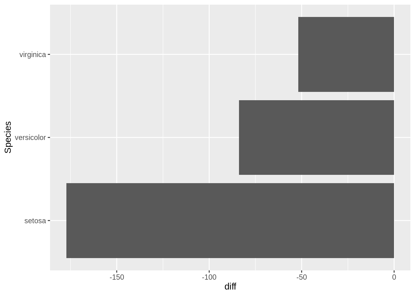
summarize
summarize is a useful function to get a new, tidy, data frame that is a summary of some other data. It's particularly useful in conjunction with group_by, when you want to compare groups.
For example, let's say you wanted to the following:
- Create a new column called
Sepal.Length.Catwith valuessmallwhenSepal.Length< 5.1,largewhenSepal.Length>= 5.8, andmediumotherwise. - Get a summary containing the average
Sepal.WidthbySepal.Length.CatandSpecies. - Get a summary containing the variation in averages for each
Species.
iris %>%
mutate(Sepal.Length.Cat = case_when(
Sepal.Length < 5.1 ~ "small",
Sepal.Length >= 5.8 ~ "large",
TRUE ~ "medium"
)) %>%
group_by(Sepal.Length.Cat, Species) %>%
summarize(avg_sepal_width_grouped = mean(Sepal.Width)) %>%
group_by(Species) %>%
summarize(std_of_avgs = sd(avg_sepal_width_grouped))## `summarise()` regrouping output by 'Sepal.Length.Cat' (override with `.groups` argument)## `summarise()` ungrouping output (override with `.groups` argument)## # A tibble: 3 x 2
## Species std_of_avgs
## <fct> <dbl>
## 1 setosa 0.402
## 2 versicolor 0.329
## 3 virginica 0.255As you can see, it has some pretty powerful functionality that would be more difficult to replicate (and harder to read) using base R.
str_extract and str_extract_all
str_extract and str_extract_all are useful functions from the stringr package. You can install the package by running:
install.packages("stringr")str_extract extracts the text which matches the provided regular expression or pattern. Note that this differs from grep in a major way. grep simply returns the index in which a pattern match was found. str_extract returns the actual matching text. Note that grep typically returns the entire line where a match was found. str_extract returns only the part of the line or text that matches the pattern. For example:
text <- c("cat", "mat", "spat", "spatula", "gnat")
# All 5 "lines" of text were a match.
grep(".*at", text)## [1] 1 2 3 4 5text <- c("cat", "mat", "spat", "spatula", "gnat")
stringr::str_extract(text, ".*at") ## [1] "cat" "mat" "spat" "spat" "gnat"As you can see, although all 5 words match our pattern and would be returned by grep, str_extract only returns the actual text that matches the pattern. In this case "spatula" is not a "full" match -- the pattern ".*at" only captures the "spat" part of "spatula". In order to capture the rest of the word you would need to add something like ".*" to the end of the pattern:
text <- c("cat", "mat", "spat", "spatula", "gnat")
stringr::str_extract(text, ".*at.*") ## [1] "cat" "mat" "spat" "spatula" "gnat"One final note is that you must double-escape certain characters in patterns because R treats backslashes as escape values for character constants (stackoverflow). For example, to write \( we must first escape the \, so we write \\(. This is true for many character which would normally only be preceded by a single \.
Examples
How can I extract the text between parenthesis in a vector of texts?
Click here for solution
text <- c("this is easy for (you)", "there (are) challenging ones", "text is (really awesome) (ok?)")
# Search for a literal "(", followed by any amount of any text other than more parenthesis ([^()]*), followed by a literal ")".
stringr::str_extract(text, "\\([^()]*\\)")## [1] "(you)" "(are)" "(really awesome)"To get all matches, not just the first match:
text <- c("this is easy for (you)", "there (are) challenging ones", "text is (really awesome) more text (ok?)")
# Search for a literal "(", followed by any amount of any text (.*), followed by a literal ")".
stringr::str_extract_all(text, "\\([^()]*\\)")## [[1]]
## [1] "(you)"
##
## [[2]]
## [1] "(are)"
##
## [[3]]
## [1] "(really awesome)" "(ok?)"lubridate
lubridate is a fantastic package that makes the typical tasks one would perform on dates, that much easier.
How do I convert a string "07/05/1990" to a Date?
Click here for solution
library(lubridate)##
## Attaching package: 'lubridate'## The following objects are masked from 'package:data.table':
##
## hour, isoweek, mday, minute, month, quarter, second, wday, week,
## yday, year## The following objects are masked from 'package:base':
##
## date, intersect, setdiff, uniondat <- "07/05/1990"
dat <- mdy(dat)
class(dat)## [1] "Date"How do I convert a string "31-12-1990" to a Date?
Click here for solution
my_string <- "31-12-1990"
dat <- dmy(my_string)
dat## [1] "1990-12-31"class(dat)## [1] "Date"How do I convert a string "31121990" to a Date?
Click here for solution
my_string <- "31121990"
my_date <- dmy(my_string)
my_date## [1] "1990-12-31"class(my_date)## [1] "Date"How do I extract the day, week, month, quarter, and year from a Date?
Click here for solution
my_date <- dmy("31121990")
day(my_date)## [1] 31week(my_date)## [1] 53month(my_date)## [1] 12quarter(my_date)## [1] 4year(my_date)## [1] 1990strrep
strrep is a function that allows you to repeat the characters a given number of times.
Examples
How to repeat the string of characters ABC three times?
Click here for solution
strrep("ABC", 3)## [1] "ABCABCABC"How to get a vector in which A is repeated twice B three times and C four times?
Click here for solution
strrep(c("A", "B", "C"), c(2,3,4))## [1] "AA" "BBB" "CCCC"nchar
nchar is a function which counts the number of characters and symbols in a word or a string. Punctuation and blank spaces are counted as well.
Examples
How to to find the number of characters and or symbols the word "Protozoa"?
Click here for solution
nchar("Protozoa")## [1] 8How to to find the number of characters and or symbols forthe following strings all at once "pneumonoultramicroscopicsilicovolcanoconiosis", "password: DatamineRocks#stat1900@"?
Fun fact: "pneumonoultramicroscopicsilicovolcanoconiosis" is the longest word in the English dictionary.
Click here for solution
string_vector <- c("pneumonoultramicroscopicsilicovolcanoconiosis", "password: DatamineRocks#stat1900@")
nchar(string_vector)## [1] 45 33Resources
A comprehensive cheatsheet on lubridate. Excellent resource to immediately begin using lubridate.